This page explains transfer function examples of common basic systems and how they are derived.
Note: If you have not learned the basics of transfer functions, please see this page first.
First-Order System
What is First-Order System?
A system whose input-output relation is expressed by a first-order linear differential equation is called a first-order system.
$$a_1 \dot{y}(t) + a_0 y(t) = b_0 u(t)$$
Organizing the Laplace transform of this equation yields the transfer function $G(s)$.
$$ Y(s) = \ubg{\frac{b_0}{a_1 s + a_0}}{\large G(s)} U(s)$$
Note that the degree of the $s$ in the denominator is 1 since this is a first-order equation.
Let’s look at examples of first-order systems and their transfer functions.
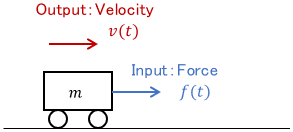
Mechanical System with Translational Motion
First, here is an example of a mechanical system.
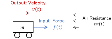
The input is the force $f(t)$ applied to the cart, the output is the velocity $v(t)$ of the cart, $m$ is the mass of the cart, and $c$ is the air resistance coefficient. The equation of motion for this cart is
$$m\dot{v}(t) = -cv(t) + f(t).$$
This is a first-order differential equation. The Laplace transform of this is
$$msV(s) = -cV(s) + F(s).$$
Organizing the equation for the output yields the transfer function $G(s)$:
$$V(s) = \ubg{\frac{1}{ms+c}}{\large G(s)} F(s)$$
Mechanical System with Rotational Motion
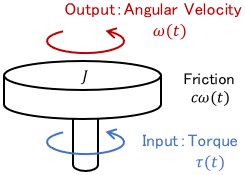
The input is the torque $\tau (t)$, the output is the angular velocity $\omega (t)$, $J$ is the moment of inertia of the disk, and $c$ is the viscous friction coefficient. The equation of motion for this disk is
$$J \dot{\omega}(t) = -c \omega(t) + \tau(t).$$
Organizing the Laplace transform of this yields the transfer function $G(s)$.
$$\begin{gather} J s\Omega(s) = -c \Omega(s) + T(s) \\[5pt] \Omega(s) = \ubg{\frac{1}{Js+c}}{\large G(s)} T(s)\end{gather}$$
This has essentially the same configuration as the previous example.
In practice, mechanical systems are most often represented as second-order systems, as we will see in the next section. However, keep in mind that systems where the input is force and the output is velocity, like the two examples above, are represented by first-order systems.
RC Circuit
An example of an electrical system is an RC circuit.
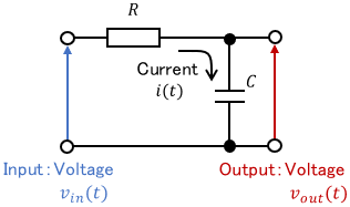
The input is the voltage $v_{in}(t)$, the output is the voltage $v_{out}(t)$, $i(t)$ is the current, $R$ is the resistance, and $C$ is the capacitance. By focusing on the capacitor, the current $i(t)$ can be derived by the following equation.
$$i(t) = C\dot{v}_{out}(t)$$
Also, the voltage applied to each element can be expressed as follows:
$$\begin{align} \text{Voltage across the resistor} &:Ri(t) \\[5pt] \text{Voltage across the capacitor} &:v_{out}(t)\end{align}$$
From Kirchhoff’s law, we can express the relation between each voltage as
$$\begin{align} v_{in}(t) &= Ri(t) + v_{out}(t) \\[5pt] &= RC \dot{v}_{out}(t)+ v_{out}(t).\end{align}$$
Organizing the Laplace transform of this yields the transfer function $G(s)$.
$$\begin{gather}V_{in}(s) = RCs V_{out}(s) + V_{out}(s) \\[5pt] V_{out}(s) = \ubg{\frac{1}{RCs + 1}}{\large G(s)} V_{in}(s)\end{gather}$$
Second-Order System
What is Second-Order System?
A system whose input-output relation is expressed by a second-order linear differential equation is called a second-order system.
$$a_2 \ddot{y}(t) + a_1 \dot{y}(t) + a_0 y(t) = b_0 u(t)$$
Organizing the Laplace transform of this equation yields the transfer function $G(s)$.
$$ Y(s) = \ubg{\frac{b_0}{a_2 s^2 + a_1 s + a_0}}{\large G(s)} U(s)$$
Note that the degree of the $s$ in the denominator is 2 since this is a second-order equation.
Then, let’s look at examples of second-order systems and their transfer functions.
Spring-Mass-Damper System
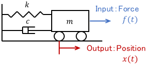
The input is the force $f(t)$ applied to the cart, the output is the position $x(t)$ of the cart, $m$ is the mass of the cart, $k$ is the spring constant, and $c$ is the viscosity coefficient. The equation of motion for this cart is
$$m\ddot{x}(t) = -c\dot{x}(t) – k x(t) + f(t).$$
Organizing the Laplace transform of this yields the transfer function $G(s)$.
$$\begin{gather}m s^2 X(s) = -c s X(s) – k X(s) + F(s)\\[5pt] X(s) = \ubg{\frac{1}{ms^2 + c s + k}}{\large G(s)} F(s)\end{gather}$$
If there is no spring or damper, just set $k$ or $c$ to 0.
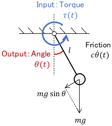
Rigid Body Pendulum
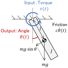
The input is the torque $\tau (t)$, the output is the angle $\theta (t)$, $J$ is the moment of inertia around the rotation axis, $m$ is the mass of the pendulum, $c$ is the viscous friction coefficient, and $g$ is the gravitational acceleration.
Considering only motion near $\theta=0$ and approximating $\sin \theta \approx \theta$, the equation of motion of the pendulum becomes
$$\begin{align} J \ddot{\theta}(t) &= -c \dot{\theta}(t) – mgl \sin \bigl( \theta(t) \bigr) + \tau(t) \\[3pt] & \approx -c \dot{\theta}(t) – mgl \theta(t) + \tau(t).\end{align}$$
Note: The Taylor series approximation around $\theta=0$ is used here. For more details on the Taylor series, please see this page:

Organizing the Laplace transform of this yields the transfer function $G(s)$.
$$\begin{gather}J s^2 \Theta (s) = -c s \Theta (s) – mgl \Theta(s) + T(s) \\[5pt] \Theta (s) = \ubg{\frac{1}{Js^2 +c s + mgl}}{\large G(s)} T(s) \end{gather}$$
Note that if the moment of inertia around the center of gravity, $J_G$, is given instead of $J$, we can convert $J_G$ to $J$ as follows and apply the above equation.
$$J=J_G+ml^2$$
Also, in the case of a simple pendulum, we can obtain the transfer function by setting $J=ml^2$.
Since the equation of motion is a second-order differential equation for position (or angle), a mechanical system where the input is force and the output is position (or angle), like the two examples above, is a second-order system.
RLC Circuit
Next is an example of an electrical system.
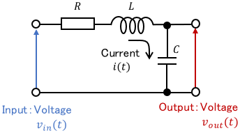
The input is the voltage $v_{in}(t)$, the output is the voltage $v_{out}(t)$, $i(t)$ is the current, $R$ is the resistance, $L$ is the inductance, and $C$ is the capacitance. By focusing on the capacitor, the current $i(t)$ can be derived by the following equation.
$$i(t) = C\dot{v}_{out}(t)$$
Also, the voltage applied to each element can be expressed as follows:
$$\begin{align} \text{Voltage across the resistor} &:Ri(t) \\[3pt] \text{Voltage across the inductor}&:L\dot{i}(t) \\[5pt] \text{Voltage across the capacitor}&:v_{out}(t)\end{align}$$
From Kirchhoff’s law, we can express the relation between each voltage as
$$\begin{align} v_{in}(t) &= Ri(t) + L\dot{i}(t) + v_{out}(t) \\[5pt] &= RC \dot{v}_{out}(t) + LC\ddot{v}_{out}(t) + v_{out}(t).\end{align}$$
Organizing the Laplace transform of this yields the transfer function $G(s)$.
$$\begin{gather}V_{in}(s) = LCs^2 V_{out}(s) + RCs V_{out}(s) + V_{out}(s) \\[5pt] V_{out}(s) = \ubg{\frac{1}{LCs^2 + RCs + 1}}{\large G(s)} V_{in}(s) \end{gather}$$
Integral System
What is Integral System?
A system whose input-output relation is expressed by a first-order linear differential equation like the following is called an integral system.
$$ \dot{y}(t) = b_0 u(t)$$
Organizing the Laplace transform of this equation yields the transfer function $G(s)$.
$$ Y(s) = \ubg{\frac{b_0}{s}}{G(s)} U(s)$$
The key point is that $\frac{1}{s}$, which represents the integration, is alone in the transfer function.
So we can obtain the solution to this equation by integrating the input without using the Laplace transform (the initial value of $y$ is assumed to be 0.)
$$ y(t) = {b_0} \int _0 ^t u(\tau) d\tau$$
Therefore, we can interpret that the integral system represents the accumulation of a given input from time to time.
Let’s look at examples of integral systems and their transfer functions.
Mechanical System with Translational Motion (without Resistance)
The input is the force $f(t)$ applied to the cart, the output is the velocity $v(t)$ of the cart, and $m$ is the mass of the cart. This is the case without air resistance in the example of the first-order system. The equation of motion for this cart is
$$m\dot{v}(t) = f(t).$$
Organizing the Laplace transform of this yields the transfer function $G(s)$.
$$\begin{gather}msV(s) = F(s) \\[5pt] V(s) = \ubg{\frac{1}{ms}}{\large G(s)} F(s) \end{gather}$$
We can interpret that the given force accumulates from time to time as kinetic energy and produces velocity.
Water Tank
Next, consider the following system in which water is supplied to a tank.
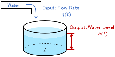
The input is the flow rate $q(t)$ (unit: $\mathrm{m^3/s}$), the output is the water level $h(t)$ (unit: $\mathrm{m}$), and $A$ is the cross-sectional area of the tank (unit: $\mathrm{m^2}$). By focusing on the change of water volume in the tank, the relation between flow rate $q(t)$ and water level $h(t)$ is expressed as follows:
$$A\dot{h}(t) = q(t)$$
Organizing the Laplace transform of this yields the transfer function $G(s)$.
$$\begin{gather} AsH(s) = Q(s) \\[5pt] H(s) = \ubg{\frac{1}{As}}{\large G(s)} Q(s) \end{gather}$$
We can interpret that the given water accumulates continuously, increasing the water level.
Heater
Consider a system where water in a tank is heated.
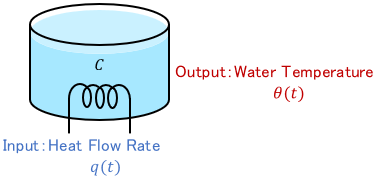
The input is the heat flow rate $q(t)$ (unit: $\mathrm{J/s}$), the output is the water temperature $\theta(t)$ (unit: $\mathrm{^\circ C}$), and $C$ is the heat capacity of water (unit: $\mathrm{J/^\circ C}$). By focusing on the change in water temperature, the relation between heat flow $q(t)$ and water temperature $\theta(t)$ can be expressed as
$$C\dot{\theta}(t) = q(t).$$
Organizing the Laplace transform of this yields the transfer function $G(s)$.
$$\begin{gather}Cs\Theta(s) = Q(s) \\[5pt] \Theta(s) = \ubg{\frac{1}{Cs}}{\large G(s)} Q(s) \end{gather}$$
We can interpret that the given heat accumulates continuously, increasing the temperature.
Proportional System
What is Proportional System?
A system whose input-output relation is proportional is called a proportional system.
$$ y(t) = K u(t)$$
The Laplace transform of this system also has the same proportional relation.
$$ Y(s) = \ubg{K}{\large G(s)} U(s)$$
Since this is not a differential equation but just an algebraic equation, the proportional element is a static system.
Note: For more details on dynamic and static systems, please see this page:
Let’s look at some examples of proportional systems.
Spring
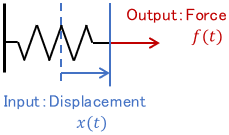
The input is the spring displacement $x(t)$, the output is the force $f(t)$, and $k$ is the spring constant. The relation between them is expressed by Hooke’s law.
$$f(t) = kx(t)$$
After the Laplace transform, the spring constant becomes the transfer function.
$$F(s) = \ubg{k}{\large G(s)}X(s)$$
Electric Resistance
Let us consider a simple voltage divider circuit.
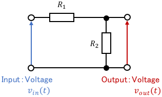
The input is the voltage $v_{in}(t)$, the output is the voltage $v_{out}(t)$, and $R_1$ and $R_2$ are resistances. The relation between them is expressed by the following equation.
$$v_{out}(t) = \frac{R_2}{R_1 + R_2} v_{in}(t)$$
In this case, the composite resistance becomes the transfer function.
$$V_{out}(s) = \ubg{\frac{R_2}{R_1 + R_2}}{\large G(s)} V_{in}(s)$$
Higher-Order Systems
Higher-order systems are complex, but it is known that most of them can be expressed as a combination of first-order, second-order, integral, and proportional systems.
Therefore, if you understand the systems and their transfer functions introduced so far, you can apply the ideas to higher-order systems. For details, please refer to this page:

Comments