This page explains the definition and advantages of the transfer function with examples. It also explains why the initial values of input and output can be considered 0 when dealing with transfer functions.
- The transfer function is a function that expresses the input-output characteristics of a system, obtained as a result of the Laplace transform.
- It is very easy to handle because the input-output relationship can be expressed simply as “output = transfer function × input.”
- A slight modification of the transfer function results in a frequency transfer function, which is useful for frequency analysis.
- Usually, the initial values of input and output (and their derivatives) are assumed to be 0. In practical use, that’s rarely a problem.
Overview of Transfer Function
The transfer function is a function that represents the input-output characteristics of a system. It is the fundamental function of classical control. Let’s look at the details.
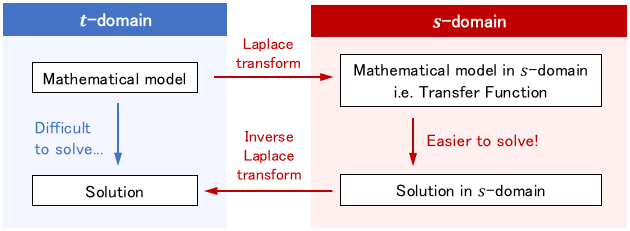
In general, a mathematical model of a dynamic system is represented by a differential equation. As the system becomes more complex, the differential equations also become more complex, and their analysis becomes difficult.
So, in classical control, the mathematical model of the system is transformed into an easy-to-handle form using a variable transformation called the Laplace transform. What is obtained in this way (i.e., the Laplace transform of the mathematical model) is the transfer function.
Note: For more details on the Laplace transform, please see this page:
Example of Transfer Function
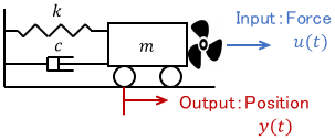
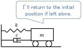
Let’s check it out with an example. Consider the following mechanical system:

The input is the force $u(t)$ acting on the cart, and the output is the position $y(t)$ of the cart. The mathematical model of this system is expressed by the equation of motion as follows.
$$m\ddot{y} + c\dot{y} + ky = u$$
Assume that the cart is initially at rest in equilibrium, i.e. \(y(0)=\dot{y}(0)=0\). Now let’s calculate the Laplace transform of this equation.
$$ms^2Y(s) + csY(s) + kY(s) = U(s)$$
where $U(s)$ and $Y(s)$ are the Laplace transforms of $u(t)$ and $y(t)$, respectively. Organizing this equation for output $Y(s)$, we obtain the following equation.
$$Y(s)=\ubg{\frac{1}{ms^2 + cs + k}}{\large G(s)} U(s)=G(s)\cdot U(s)$$
In the $s$-domain, the output is represented in the form “function $G(s)$ × input $U(s)$.” This function $G(s)$ connecting the input and output is the transfer function!
$$\usg{Y(s)}{\text{Output}} = \usgd{G(s)}{\text{Transfer}}{\text{Funciton}} \cdot \usg{U(s)}{\text{Input}} $$
Next, let’s take a closer look at the advantages of the transfer function.
Advantages of Transfer Function
Advantage 1: Differential equations can be solved with multiplication!
As shown in the previous example, the transfer function allows us to obtain the output by simply multiplying the transfer function and the input.
Usually, solving differential equations requires tedious integral operations. It is a great help if the integration becomes a multiplication, isn’t it?
With the transfer function, even higher-order differential equations can be solved by multiplication only. Therefore, the more complex the system is, the greater the benefit becomes.
$$y^{(4)}+a_3 y^{(3)}+ a_2 y^{(2)}+ a_1 y^{(1)} +a_0 y = b_1 u^{(1)} + b_0 u$$
$$Y(s) =\ubgd{ \frac{b_1 s + b_0}{s^4 + a_3 s^3 + a_2 s^2 + a_1 s + a_0}U(s)}{\large \text{No matter how many derivatives,}}{\large \text{just multiply them to get the output!}}$$
Here, the solution $y(t)$ in the $t$-domain can be obtained by finding the inverse Laplace transform of $Y(s)$.
Note: For more information on how to solve differential equations using the Laplace transform, please see this page:
Also, by looking at the poles and zeros of the transfer function, we can easily analyze the behavior of $y(t)$ without the inverse Laplace transform. Such ease of use is a major advantage of the transfer function.
Advantage 2: Systems can be combined easily!
In the previous system, we assumed that the input force $u$ could be freely given. Now let us assume that the force is generated by the wind from a propeller, as shown in the figure below.
Let us consider the system characteristics, including those of the propeller. Suppose that the propeller generates wind force $u$ in response to the input current $i$, which is described by the following differential equation:
$$\ddot{u} + a_1 \dot{u} + a_0 u= i$$
The block diagram of the system looks like this.
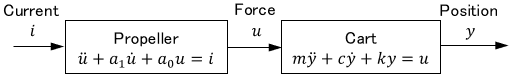
Thus, to obtain the motion $y$, we must first solve the differential equation for the propeller and then solve the differential equation for the cart using its solution $u$ as input.
Of course, such a calculation is possible, but it is tedious and does not give a clear view of the entire system’s characteristics. This is even more so for a more complex system.
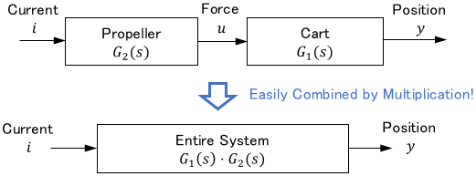
Transfer functions can also easily handle such cases. Since input and output have a multiplicative relationship in the s-domain, we can obtain the input-output characteristics of the entire system (from $i$ to $y$) by multiplying the transfer functions as follows:
$$\begin{align} \text{Cart Characteristics:}\quad Y(s)&=\frac{1}{ms^2 + cs + k}U(s)\\ \\ \text{Propeller Characteristics:}\quad U(s) &=\frac{1}{s^2 + a_1s + a_0}I(s) \\\\ \text{Entire Characteristics:}\quad Y(s)&=\ubg{\frac{1}{ms^2 + cs + k}}{\large \text{Cart }G_1(s)} \cdot \ubg{\frac{1}{s^2 + a_1s + a_0}}{\large \text{Propeller }G_2(s)} I(s)\end{align}$$
Advantage 3: Frequency analysis with ease!
Since Laplace transform is very compatible with frequency analysis, we can easily perform frequency analysis of a system using transfer functions.
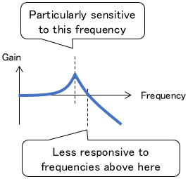
Frequency analysis is a technique for analyzing how a system responds to various frequency signal components. (Think of frequency as how fast a signal changes.)
It allows us to obtain information about a target system, such as “particularly sensitive to this frequency” or “less responsive to frequencies above here.”
Let’s return to the transfer function. Let $\omega$ be the frequency and $j$ the imaginary unit. It is known that $G(\omega j)$, where $\omega j$ is assigned to the transfer function $G(s)$, represents the frequency response of the system.
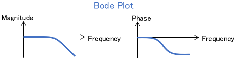
By using the frequency response, we can easily perform frequency analysis. For example, by drawing $G(\omega j)$ in terms of $\omega$, a Bode diagram is obtained. This allows us to check the frequency response of the system visually.
The reason why the initial values can be considered 0
In classical control, systems are handled by assuming that the initial values of input and output (and their derivatives) are all 0 in most cases. We have made this assumption in the examples so far.
We make this assumption because, in the s-domain, the time differentiation becomes very simple and easy to handle, as follows:
$$\begin{alignat}{2}\dot{f}(t) &\ \xrightarrow{ \text{Laplace transform}} \ sF(s) – f(0) &&= sF(s) \\[3px] \ddot{f}(t) &\ \xrightarrow{\text{Laplace transform}} \ s^2 F(s) -sf(0) – \dot{f}(0) &&= s^2 F(s)\end{alignat}$$
Can we make such assumptions on our own?
Doesn’t it narrow the scope of the application?
In fact, it is not much of a problem in most cases. Let’s take a closer look at the reasons for this.
Reason 1: In most cases, the initial value is actually 0
For most systems, an initial value of 0 means that the system is initially stopped or at the equilibrium point. Most systems start moving from either of these states, so most of the time the initial values are actually 0.
For example, in a mechanical system, this would be the state where the system stops in the balanced position. Naturally, we turn on the switch and move it from this state.
Even if the system is running, we can easily reset it to 0 by turning it off. Therefore, for practical use, there is little trouble in assuming that the initial values are 0.
Reason 2: Transfer function does not change regardless of the initial values
If the actual initial values are not 0, the calculated output $Y(s)$ will differ from the actual behavior. Even in such a case, it is not a problem in terms of controller design in most cases. Let us look at this in detail.
Controller design in classical control is mostly based on the relationship between inputs and outputs, i.e. how the inputs affect the outputs, rather than on what exactly the outputs will be. For example, the frequency analysis introduced earlier is a method to analyze the input-output relationship, not the specific output behavior, right?
And, in fact, the transfer function, which represents the input-output relationship, does not change regardless of the initial values. Therefore, in most cases, a controller can be designed appropriately even if the initial values differ from reality.
As an example, let’s consider again the mechanical system described earlier.
$$m\ddot{y} + c\dot{y} + ky = u$$
We will calculate the Laplace transform of the equation without taking the initial values $y(0)$ and $\dot{y}(0)$ as 0.
$$m\bigl\{ s^2Y(s) -sy(0) – \dot{y}(0) \bigr\} + c\bigl\{ sY(s) – y(0)\bigr\} + kY(s) = U(s)$$
The output can be expressed as follows:
$$Y(s)= \ubg{\frac{1}{ms^2 + cs + k}}{\large G(s)} \Bigl[ U(s) + \ubg{\vphantom{ \frac{1}{ms^2 + cs + k} }m\bigl\{ sy(0) + \dot{y}(0)\bigr\} + dy(0)}{\large I(s)\text{: Initial Value Terms}} \Bigr]$$
If we let $I(s)$ be the term related to the initial values, we can see that $I(s)$ and the input $U(s)$ act independently on the output $Y(s)$.
$$\begin{align}\osg{Y(s)}{\text{Output}} &= \osgd{G(s)}{\text{Transfer}}{\text{Function}} \Bigl\{ \osg{U(s)}{\text{Input}} + \osgd{I(s)}{\text{Initial}}{\text{Terms}} \Bigr\} \\[3pt] &= G(s)U(s) + G(s) I(s) \end{align}$$
Therefore, the transfer function $G(s)$ can represent the input-output relationship even when the initial value is not 0.
This page explained the definition and advantages of the transfer function with examples. Please also see the page below for many concrete examples of transfer functions.
- The transfer function is a function that expresses the input-output characteristics of a system, obtained as a result of the Laplace transform.
- It is very easy to handle because the input-output relationship can be expressed simply as “output = transfer function × input.”
- A slight modification of the transfer function results in a frequency transfer function, which is useful for frequency analysis.
- Usually, the initial values of input and output (and their derivatives) are assumed to be 0. In practical use, that’s rarely a problem.
Comments