This page explains the steady-state error and internal model principle when a disturbance acts on a feedback control system.
Note: This page is a continuation of the page below. If you have not yet learned about the steady-state error and internal model principles, please see this first.

- If the feedback controller has the same number of integrators as the disturbance, the disturbance effect becomes zero.
- In other words, the internal model principle also holds for disturbances.
- Even if integrators are insufficient, the disturbance effect can be reduced by increasing the control gain.
Calculation of Steady-State Error by Disturbance
Derivation with Final Value Theorem
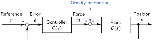
Consider the following case where a disturbance acts on a feedback control system.
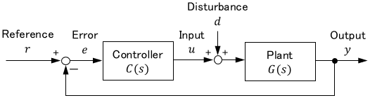
where $C(s)$ is the transfer function of the controller and $G(s)$ is the transfer function of the plant.
We will calculate the steady-state error $e_s$ under the above condition. The steady-state error can be calculated with the final value theorem of the Laplace transform as follows.
$$e_s = \lim _{t\rightarrow \infty} e(t) = \lim _{s\rightarrow 0} sE(s)$$
where $E(s)$ is the Laplace transform of the error $e(t)$. The $E(s)$ can be obtained from the relation on the block diagram as follows:
$$\begin{align}\text{From relation on block diagram}, \quad & E(s) = R(s) – Y(s)\\[8pt] \text{By expressing }Y(s)\text{ in terms of }E(s) \text{ & } D(s), \quad & E(s) = R(s) – G(s)\bigr\{C(s)E(s)+D(s)\bigl\}\\[3pt] \text{By organising for }E(s), \quad & E(s) = \ubgd{\frac{1}{1 + C(s)G(s)} R(s)}{\large \quad R(s) \text{ term.}}{\large \text{Same as last time}} – \ubgd{\frac{G(s)}{1+C(s)G(s)}D(s)}{\large \qquad D(s) \text{ term.}}{\large \text{Effect of disturbance}} \end{align}$$
where $R(s)$ is the Laplace transform of the reference $r(t)$, $Y(s)$ is the Laplace transform of the output $y(t)$, and $D(s)$ is the Laplace transform of the disturbance $d(s)$. The term with the reference $R(s)$ is the same as on the previous page. In addition, the term with the disturbance $D(s)$ has appeared.
By substituting this into the previous equation, we obtain the steady-state error as follows:
$$e_s = \lim _{s\rightarrow 0} sE(s) = \lim _{s\rightarrow 0} \Biggl\{\ubgd{s \cdot\frac{1}{1 + C(s)G(s)} R(s)}{\large \quad R(s) \text{ term.}}{\large \text{Same as last time}} – \ubgd{s \cdot\frac{G(s)}{1+C(s)G(s)}D(s)}{\large \qquad D(s) \text{ term.}}{\large \text{Effect of disturbance}}\Biggr\}$$
So, for the steady-state error to be zero, not only the $R(s)$ term but also the $D(s)$ term must be zero. The idea for the $R(s)$ term is the same as on the previous page, so let’s leave it aside and consider the $D(s)$ term.
Steady-State Error against Step Disturbance
Consider the case where a unit step disturbance $D(s)=\frac{1}{s}$ acts.

In this case, the $D(s)$ term becomes as follows:
$$D(s)\text{ term}=\lim _{s\rightarrow 0}s \cdot\frac{G(s)}{1+C(s)G(s)}\cdot \ubg{\frac{1}{s}}{\large \text{Step}}=\lim _{s\rightarrow 0}\frac{G(s)}{1+C(s)G(s)}$$
Therefore, to make this term zero, $G(s)$ must be zero, or $C(s)$ must be $\infty$ with $s\rightarrow 0$.
$$D(s)\text{ term}=\lim _{s\rightarrow 0}\frac{\obg{G(s)}{\large 0 \text{ here,}}}{1+\ubgd{C(s)}{\large \quad \text{or}}{\large \infty \text{ here}}G(s)}$$
Note: If only $G(s)$ goes to $\infty$, it converges to $\frac{1}{C(0)}$.
For this to be satisfied, the plant $G(s)$ needs to have differentiator $s$, or the controller $C(s)$ needs to have an integrator $\frac{1}{s}$.
Since proper systems, which are mainly handled in classical control, cannot have a differentiator, it is important for practical purposes that the controller $C(s)$ have an integrator.
Note: For more information on the relation between proper systems and differentiators, please see this page:

So, for the step disturbance $\frac{1}{s}$, $C(s)$ needs to have $\frac{1}{s}$. This is a similar result to the one on the previous page.
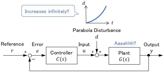
The same discussion yields similar results for ramp and parabola disturbances. (If you have time, please try the calculations).

In other words, the internal model principle holds for disturbances as well.
Summary of Internal Model Principle
By integrating the discussion on the previous page and this page, the internal model principle can be summarized as follows:
- For the reference $R(s)=\frac{1}{s^k}$, the steady-state error becomes zero if $C(s)G(s)$ has $\frac{1}{s^k}$.
- If the disturbance $D(s)=\frac{1}{s^k}$ acts, its effect becomes zero if $C(s)$ has $\frac{1}{s^k}$.
Note that $C(s)G(s)$ is the target for the reference, but $C(s)$ alone is the target for the disturbance. This means that if the control plant $G(s)$ originally has integrators, the number of integrators needed by the controller $C(s)$ will be different for each.
After all, we cannot go wrong if $C(s)$ has integrators, but note that increasing the integrators will make the system less stable, as explained on the previous page.
Simulation Examples
Now let’s see if the above really holds by simulations.
As an example, consider the following system given a step reference $R(s)=\frac{1}{s}$ and a step disturbance $D(s)=\frac{1}{s}$.

Note that the plant $G(s)=\frac{2s+1}{s^2+2s+3}$ has no integrator. Let us add some integrators with the following controllers and compare the steady-state error.
$$\begin{array}{lll} \text{With }C(s) = K_0,& C(s)G(s) \text{ has }\color{red}{\mathbf{0}} \text{ integrators.} \\[5pt] \text{With }C(s) = \frac{K_1}{s}, & C(s)G(s) \text{ has }\color{red}{\mathbf{1}} \text{ integrator.} \\[5pt] \text{With }C(s) = \frac{K_2}{s^2}, & C(s)G(s) \text{ has }\color{red}{\mathbf{2}} \text{ integrators.}\end{array}$$
where $K_0$, $K_1$, and $K_2$ are constant control gains (i.e. tuning parameters). Simulation with appropriate gains yields the following results.

As the internal model principle says, when the controller $C(s)$ has one or more integrators, the disturbance effect is canceled out, and the steady-state error becomes zero.
In contrast, the constant steady-state error remains if the controller has no integrator. Further observation shows that the steady-state error is smaller when the control gain $K_0$ is larger.
Let us check these with equations. The steady-state error $e_s$ for $C(s)=K_0$ is calculated as follows. (You can skip the calculation process.)
$$\text{By using }\ e_s = \lim _{s\rightarrow 0} \Biggl\{s \cdot\frac{1}{1 + C(s)G(s)} R(s) – s \cdot\frac{G(s)}{1+C(s)G(s)}D(s)\Biggr\}\ \text{ and }\ C(s)=K_0,$$
$$ e_s = \lim _{s\rightarrow 0} \Biggl\{\ubg{s \cdot\frac{1}{1 + K_0\frac{2s+1}{s^2+2s+3} } \cdot \frac{1}{s}}{\large R(s)\text{ term}}\ -\ \ubg{s \cdot\frac{ \frac{2s+1}{s^2+2s+3} }{1+ K_0\frac{2s+1}{s^2+2s+3} } \cdot \frac{1}{s}}{\large D(s)\text{ term}} \Biggr\} = \ubg{\frac{1}{1 + \frac{K_0}{3} }}{\large R(s)\text{ term}}+\ubg{\frac{\frac{1}{3}}{1+\frac{K_0}{3}}}{\large D(s)\text{ term}}$$
For both the $R(s)$ and $D(s)$ terms, we can see that the larger the control gain $K_0$, the larger the denominators, resulting in a smaller steady-state error.
Therefore, even in the presence of disturbance, if the integrator is insufficient, we can reduce the disturbance effect by increasing the control gain as much as possible.
Practical Tips on Disturbances
Seldom Used Except Step Disturbance
As mentioned earlier, the effects of ramp and parabola disturbances can also be eliminated by adding integrators based on the internal model principle.
For practical use, however, only the step disturbance is almost always used. Although the ramp and parabola disturbances increase infinitely with time, such disturbances are rarely present in reality.
Concept of Step Disturbance
What exactly is the “step disturbance”?
This can be imagined as a constant effect that always acts on the system. For example, in a mechanical system, it is the gravitational or frictional force that always works on the system.
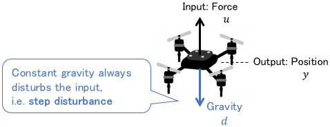

On the block diagram, these forces do indeed act as an addition to the input (i.e. as a disturbance).
Even if the cause is unclear, step disturbances can be used to represent “input deviations” resulting from various causes.

We can see the convenience of the internal model principle by considering that, whatever the cause, we can eliminate a constant input deviation by adding an integrator to the controller.
- If the feedback controller has the same number of integrators as the disturbance, the disturbance effect becomes zero.
- In other words, the internal model principle also holds for disturbances.
- Even if integrators are insufficient, the disturbance effect can be reduced by increasing the control gain.
Comments