
This page explains the steady-state characteristics of the system and how they are calculated, with examples. In particular, the internal model principle and steady-state error of a feedback control system will be discussed in detail.
- If the feedback control system has the same number of integrators as the reference, the steady-state error becomes zero.
- This is called the internal model principle.
- However, the more integrators the system has, the less stable it becomes.
- Even if integrators are insufficient, increasing the control gain can reduce the steady-state error.
Overview of Steady-State Error
What is Steady-State Error?
Steady-state error is the error in the steady-state, i.e. after the system has been operating for a sufficient period.
Especially for feedback control systems, it is very important that the controlled variable follows the reference without error. Steady-state error is used to evaluate such performance.

We can calculate steady-state error by solving the mathematical model of the system (i.e. transfer function). But, the more complex the system, the more cumbersome the calculation becomes.
Thus, classical control uses the final value theorem, a convenient property of the Laplace transform, to alleviate this problem. The final value theorem enables us to calculate steady-state error without solving a mathematical model.
Hereafter, we will focus on the steady-state error of a feedback control system and its characteristics.
Note: When discussing steady-state characteristics, it is assumed that the considered system is stable. This is because the system will not settle into a steady state if it is not stable. For more details on stability, please see this page:

Test Waveforms for Reference
When evaluating the steady-state error of a feedback system, the following test waveforms are usually used as the basic elements of the reference.

In particular, the step reference is a basic reference used very often in practical situations.
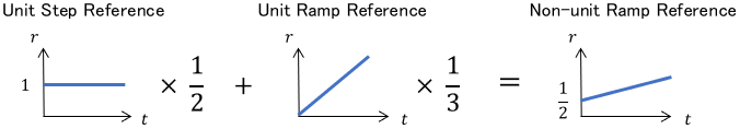
Hereafter, the “unit references,” which unify the coefficients to 1, will be used to keep the formulas clear. The formula $r(t)$ and its Laplace transform $R(s)$ for each reference are shown below.
$$\begin{array}{lll} \text{Unit Step Reference} & r(t)=1 & R(s) = \frac{1}{s} \\[2pt] \text{Unit Ramp Reference} & r(t) = t & R(s) = \frac{1}{s^2} \\ \text{Unit Parabola Reference} & r(t) = \frac{t^2}{2} & R(s) = \frac{1}{s^3}\end{array}$$
Since a combination of the unit references can express non-unit references, it is eventually sufficient to examine the characteristics against the unit references only.
Calculation of Steady-State Error
Let’s now calculate the steady-state error against each reference and look at its characteristics.
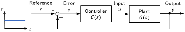
Consider the feedback control system represented by the following block diagram.

where $C(s)$ is the transfer function of the controller and $G(s)$ is the transfer function of the plant.
Derivation with Final Value Theorem
The steady-state error $e_s$ can be expressed by the following formula:
$$e_s = \lim _{t\rightarrow \infty} e(t)$$
We could calculate this directly, but with the final value theorem of the Laplace transform, we can calculate it in the $s$-domain. This means since $e_s$ can be computed with the transfer function representation, we can analyze it without tedious inverse Laplace transforms.
$$\text{Final Value Theorem: }\ \lim _{t\rightarrow \infty} f(t) = \lim _{s\rightarrow 0} s F(s)$$
where $F(s)$ is the Laplace transform of $f(t)$. It means that if we multiply the Laplace transform $F(s)$ by $s$ and apply $s \rightarrow 0$ instead of $t\rightarrow \infty$, we get the same solution as in the original equation.
Note: For the basics of the Laplace transform, please see this page:
By using this to compute the steady-state error described earlier, we obtain
$$e_s = \lim _{t\rightarrow \infty} e(t) = \lim _{s\rightarrow 0} sE(s)$$
where $E(s)$ is the Laplace transform of the error $e(t)$.
Now let’s calculate $E(s)$ in the equation. From the relationship on the block diagram, $E(s)$ is obtained as follows:
$$\begin{align}\text{From relation on block diagram}, \quad & E(s) = R(s) – Y(s)\\[8pt] \text{By expressing }Y(s)\text{ in terms of }E(s), \quad & E(s) = R(s) – C(s)G(s)E(s)\\[3pt] \text{By organising for }E(s), \quad & E(s) = \frac{1}{1 + C(s)G(s)} \cdot R(s) \end{align}$$
where $R(s)$ and $Y(s)$ are the Laplace transforms of the reference $r(t)$ and the output $y(t)$, respectively.
By substituting this into the previous equation, we obtain the formula for the steady-state error $e_s$.
$$e_s = \lim _{s\rightarrow 0} sE(s) = \lim _{s\rightarrow 0} s \cdot \frac{1}{1 + C(s)G(s)}\cdot R(s)$$
Let’s use this to calculate the steady-state error for each reference.
Steady-State Error against Step Reference
Consider the case where the unit step reference $R(s)=\frac{1}{s}$ is given as the reference.
The steady-state error $e_s$ in this case can be calculated as follows:
$$e_s = \lim _{s\rightarrow 0} s \cdot \frac{1}{1 + C(s)G(s)} \cdot \ubg{\frac{1}{s}}{\large \text{Step}} = \lim _{s\rightarrow 0} \frac{1}{1 + C(s)G(s)} $$
We see that the $s$ multiplied by the final value theorem is cancelled out by the step reference $\frac{1}{s}$.
The control objective is to achieve $e_s=0$. To do so, we want the open-loop transfer function $C(s)G(s)$ to be $\infty$ with $s\rightarrow 0$.
$$e_s = \lim _{s\rightarrow 0} \frac{1}{1 + \ubgd{C(s)G(s)}{\large \text{If this becomes}}{\large \infty\text{, then }e_s=0} }$$
Such is the case when $C(s)G(s)$ has one (or more) integrator $\frac{1}{s}$.
$$C(s)G(s) = \ubgd{\frac{1}{s}}{\large \text{Becomes}}{\large \quad\ \infty} \cdot \ubgd{L(s)\vphantom{\frac{1}{s}}}{\large \text{Other}}{\large \text{ parts}}$$
So the integrator diverges to $\infty$ with $s\rightarrow 0$. Keep in mind that “for a step reference $\frac{1}{s}$, we need $\frac{1}{s}$,” and go on.
Note: $C(s)G(s)$ is assumed to be in irreducible form. For example, $\frac{1}{s}\cdot\frac{s}{s+1}$ looks like it has an integrator, but it does not actually have one because its reduction results in $\frac{1}{s+1}$.
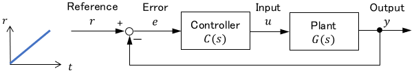
Steady-State Error against Ramp Reference
Consider the case where the unit ramp reference $R(s)=\frac{1}{s^2}$ is given as the reference.
The steady-state error $e_s$ can be calculated in the same way.
$$e_s = \lim _{s\rightarrow 0} s \cdot \frac{1}{1 + C(s)G(s)} \cdot \ubg{\frac{1}{s^2}}{\large \text{Ramp}} = \lim _{s\rightarrow 0} \frac{1}{s + sC(s)G(s)} $$
The denominator degree is one degree larger than before. To have $e_s=0$, we need $sC(s)G(s)$ to be $\infty$ with $s\rightarrow 0$.
$$e_s = \lim _{s\rightarrow 0} \frac{1}{\ubg{s}{\large \text{Will be }0} + \ubgd{sC(s)G(s)}{\large \text{If this becomes}}{\large \infty\text{, then }e_s=0} }$$
Considering similarly to before, $C(s)G(s)$ needs two (or more) integrators $\frac{1}{s}$.
$$C(s)G(s) = \ubgd{\frac{1}{s}}{\large \text{Deletes }s}{\large \text{ in front}}\cdot \obgd{\frac{1}{s}}{\large \text{Becomes}}{\large \quad \ \infty} \cdot \ubgd{L(s)\vphantom{\frac{1}{s}}}{\large \text{Other}}{\large \text{ parts}}$$
So the first integrator cancels the preceding $s$, and the second integrator diverges to $\infty$ with $s\rightarrow 0$. Keep in mind that “for a ramp reference $\frac{1}{s^2}$, we need $\frac{1}{s^2}$,” and go on.
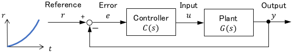
Steady-State Error against Parabola Reference
Finally, consider the case where the unit ramp reference $R(s)=\frac{1}{s^2}$ is given as the reference.
The steady-state error $e_s$ in this case can be calculated as follows:
$$e_s = \lim _{s\rightarrow 0} s \cdot \frac{1}{1 + C(s)G(s)} \cdot \ubg{\frac{1}{s^3}}{\large \text{Parabola}} = \lim _{s\rightarrow 0} \frac{1}{s^2 + s^2C(s)G(s)} $$
The denominator degree is one degree larger again. To have $e_s=0$, we need $s^2C(s)G(s)$ to be $\infty$ with $s\rightarrow 0$.
$$e_s = \lim _{s\rightarrow 0} \frac{1}{\ubg{s^2}{\large \text{Will be }0} + \ubgd{s^2C(s)G(s)}{\large \text{If this becomes}}{\large \infty\text{, then }e_s=0}} $$
You may already know what to do. $C(s)G(s)$ needs three (or more) integrators $\frac{1}{s}$, right?
$$C(s)G(s) = \ubgd{\frac{1}{s^2}}{\large \text{Deletes }s^2}{\large \text{ in front}}\cdot \obgd{\frac{1}{s}}{\large \text{Becomes}}{\large \quad \ \infty} \cdot \ubgd{L(s)\vphantom{\frac{1}{s}}}{\large \text{Other}}{\large \text{ parts}}$$
Keep in mind that “for a parabola reference $\frac{1}{s^3}$, we need $\frac{1}{s^3}$,” and go on.
Internal Model Principle
We have looked at steady-state error against the step, ramp, and parabola references. With similar discussions, the same laws hold for higher-degree references.
- For $R(s)=\frac{1}{s}$, the steady-state error becomes zero if $C(s)G(s)$ has $\frac{1}{s}$.
- For $R(s)=\frac{1}{s^2}$, the steady-state error becomes zero if $C(s)G(s)$ has $\frac{1}{s^2}$.
- For $R(s)=\frac{1}{s^3}$, the steady-state error becomes zero if $C(s)G(s)$ has $\frac{1}{s^3}$.
- For $R(s)=\frac{1}{s^k}$, the steady-state error becomes zero if $C(s)G(s)$ has $\frac{1}{s^k}$.
From the above, we can see that to achieve a steady-state error of zero, the open-loop transfer function $C(s)G(s)$ needs to have the same number of integrators as the reference.
This law is called the internal model principle. Easy to remember!
Simulation Examples
Considered System
Now let’s see if the internal model principle really holds by simulations.
As an example, consider the following system:

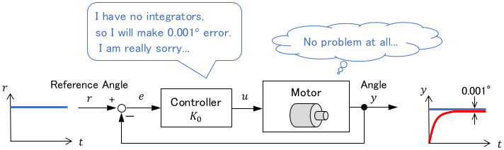
Note that the plant $G(s)=\frac{2s+1}{s^2+2s+3}$ has no integrator. Let us add some integrators with the following controllers and compare the steady-state errors.
$$\begin{array}{lll} \text{With }C(s) = K_0,& C(s)G(s) \text{ has }\color{red}{\mathbf{0}} \text{ integrators.} \\[5pt] \text{With }C(s) = \frac{K_1}{s}, & C(s)G(s) \text{ has }\color{red}{\mathbf{1}} \text{ integrator.} \\[5pt] \text{With }C(s) = \frac{K_2}{s^2}, & C(s)G(s) \text{ has }\color{red}{\mathbf{2}} \text{ integrators.}\end{array}$$
where $K_0$, $K_1$ and $K_2$ are constant control gains (i.e. tuning parameters).
Note: In this case, the controllers are composed only of integrators for clarity. In practice, however, this is rarely done, i.e. the integrator is most often used with other control elements.
Simulation with Step Reference
First, let’s simulate with the unit step reference $R(s)=\frac{1}{s}$.
According to the internal model principle, for the step reference $\frac{1}{s}$, the open-loop transfer function $C(s)G(s)$ needs one (or more) integrator. Let’s check this out.
Here are the simulation results with appropriate $K_0$, $K_1$ and $K_2$.
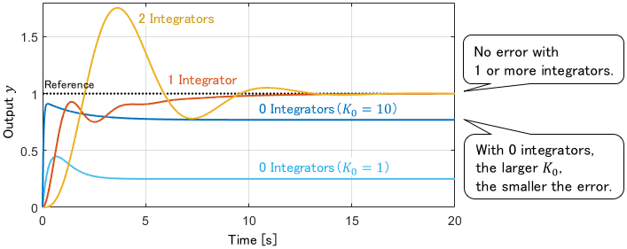
Certainly, the steady-state error becomes zero when the controller has one or more integrators.
In contrast, the constant steady-state error remains if the controller has no integrator. Further observation shows that the steady-state error is smaller when the control gain $K_0$ is larger.
Let us check these with equations. The steady-state error $e_s$ for each controller is calculated as follows. (You can skip the calculation process.)
$$\text{By using}\quad e_s =\lim _{s\rightarrow 0} s \cdot \frac{1}{1 + C(s)G(s)} \cdot R(s),$$
$$\begin{alignat}{3} &\text{With }C(s) = K_0, &&\quad e_s = \lim _{s\rightarrow 0} s \cdot \frac{1}{1 + K_0\frac{2s+1}{s^2+2s+3}} \cdot \frac{1}{s} = \frac{1}{1 + \frac{K_0}{3}}&&\quad\color{green}{\text{Certainly constant!}}\\[7pt] &\text{With }C(s) = \frac{K_1}{s}, &&\quad e_s = \lim _{s\rightarrow 0} s \cdot \frac{1}{1 + \frac{K_1}{s}\cdot\frac{2s+1}{s^2+2s+3}} \cdot \frac{1}{s} = 0 && \quad \color{green}{\text{Certainly 0!}}\\[7pt] &\text{With }C(s) = \frac{K_2}{s^2}, && \quad e_s = \lim _{s\rightarrow 0} s \cdot \frac{1}{1 + \frac{K_2}{s^2}\cdot \frac{2s+1}{s^2+2s+3}} \cdot \frac{1}{s} = 0&& \quad \color{green}{\text{Certainly 0!}}\end{alignat}$$
For $C(s)=K_0$, i.e. zero integrators, we can see that the larger the control gain $K_0$, the larger the denominator of $e_s$, resulting in a smaller steady-state error.
Therefore, if the integrator is insufficient, we can reduce the steady-state error by increasing the control gain as much as possible.
Note: The higher the control gain, the greater the risk of input saturation (i.e. demanding more than system capability). For example, if we set $K_0=\infty$, the system cannot achieve that, of course. Therefore, the gain must be adjusted within the system’s capability.
Simulation with Ramp Reference
Next, let’s simulate with the unit ramp reference $R(s)=\frac{1}{s^2}$.
According to the internal model principle, for the ramp reference $\frac{1}{s^2}$, the open-loop transfer function $C(s)G(s)$ needs two (or more) integrators.
Here are the simulation results with appropriate $K_0$, $K_1$ and $K_2$.
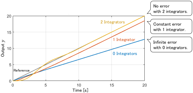
Certainly, the steady-state error becomes zero when the controller has two integrators.
In contrast, the constant steady-state error remains with one integrator, and the error has grown infinitely over time with zero integrators.
Let’s also check these with equations. The steady-state error $e_s$ for each controller is calculated as follows. (Again, you can skip the calculation process.)
$$\text{By using}\quad e_s =\lim _{s\rightarrow 0} s \cdot \frac{1}{1 + C(s)G(s)} \cdot R(s),$$
$$\begin{alignat}{3} &\text{With }C(s) = K_0, &&\quad e_s = \lim _{s\rightarrow 0} s \cdot \frac{1}{1 + K_0\frac{2s+1}{s^2+2s+3}} \cdot \frac{1}{s^2} = \infty &&\quad\color{green}{\text{Certainly }\infty\text{!}}\\[7pt] &\text{With }C(s) = \frac{K_1}{s}, &&\quad e_s = \lim _{s\rightarrow 0} s \cdot \frac{1}{1 + \frac{K_1}{s}\cdot\frac{2s+1}{s^2+2s+3}} \cdot \frac{1}{s^2} = \frac{1}{1 + \frac{K_1}{3}} &&\quad \color{green}{\text{Certainly constant!}}\\[7pt] &\text{With }C(s) = \frac{K_2}{s^2}, &&\quad e_s = \lim _{s\rightarrow 0} s \cdot \frac{1}{1 + \frac{K_2}{s^2}\cdot \frac{2s+1}{s^2+2s+3}} \cdot \frac{1}{s^2} = 0&& \quad\color{green}{\text{Certainly 0!}}\end{alignat}$$
The results of the calculations are indeed consistent with the simulation. For $C(s) = \frac{K_1}{s}$, i.e. one integrator, the same logic as before also shows that the larger the control gain $K_1$, the smaller the steady-state error.
Simulation with Parabola Reference
Next, let’s simulate with the unit parabola reference $R(s)=\frac{1}{s^3}$.
According to the internal model principle, for the parabola reference $\frac{1}{s^3}$, the open-loop transfer function $C(s)G(s)$ needs three (or more) integrators.
Here are the simulation results with appropriate $K_0$, $K_1$ and $K_2$.
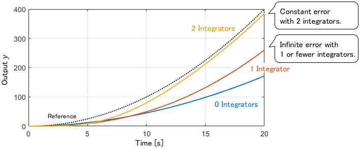
As before, the constant steady-state error remains with two integrators, and the error grows infinitely over time with one or fewer integrators.
So, with three integrators, will the steady-state error be eliminated? Here are the simulation results with three integrators.
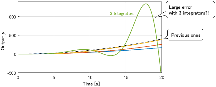
My goodness, rather than the steady-state error disappearing, it has diverged! Why does the internal model principle not hold? Let’s take a look at the reasons for this.
Stability and Practical Tips
The reason for the divergence is that the system became unstable because too many integrators were added. (Conversely, if the system remains stable, the steady-state error will properly disappear.)
As mentioned earlier, when discussing steady-state characteristics, system stability is a prerequisite. Since the internal model principle and the final value theorem are theories that assume a stable system, the calculations become meaningless if this assumption is violated.
Why does adding an integrator make the system less stable?
Since the pole of an integrator $\frac{1}{s}$ is zero, a single integrator is not a stable system. Therefore, it can be interpreted that the more integrators we add to the system, the less stable it becomes.

So how many can I put on?
It depends on the stability margin of the system. Therefore, it should be determined case-by-case basis, depending on the system.
Nevertheless, in most cases, only two or fewer integrators are used in practice. You can think of 0 integrators in general, 1 integrator if the steady-state error is too large, and 2 integrators if there is a special reason to use them.
Wait, but wouldn’t a small number of integrators result in a steady-state error?
That is correct. However, as mentioned above, we can reduce the steady-state error by increasing the control gain. So, if sufficient accuracy can be achieved by adjusting the gain, there is no need to bother adding an unstable integrator.
Thus, please note that the internal model principle is only a condition for a steady-state error to be exactly zero.
It is known that the internal model principle is also valid against a disturbance. Please refer to the page below for a detailed explanation.

- If the feedback control system has the same number of integrators as the reference, the steady-state error becomes zero.
- This is called the internal model principle.
- However, the more integrators the system has, the less stable it becomes.
- Even if integrators are insufficient, increasing the control gain can reduce the steady-state error.
Comments