This page explains the differences between linear and nonlinear systems, and between time-variant and time-invariant systems. In addition, examples of each system and their practical uses are also explained.
- A linear system is one whose mathematical model is expressed only in terms of “coefficient × input/output(s derivative),” while other systems are nonlinear systems.
- A time-invariant system is one whose coefficients are all constants. A time-variant system is one whose coefficients are time-dependent.
- Linear systems are easy to handle. Nonlinear systems are more difficult to handle.
- Time-invariant systems are easy to handle. Time-variant systems are more difficult to handle.
Linear and Nonlinear Systems
A system whose mathematical model is expressed only in terms of “coefficient × input/output(s derivative)” is called a linear system, while other systems are called nonlinear systems. The following is an example where the input is $u$, and the output is $y$.
$$ \begin{alignat}{5} a_2 \ddot{y} &\ +\ a_1 \dot{y} & &\ +\ a_0 y & &=\ b_1 \dot{u} & &\ +\ b_0 u :& & \quad \textbf{Linear}\\ a_2 \ddot{y} &\ +\ a_1 \dot{y} & &\ +\ a_0 \color{red}{\sin y }& &=\ b_1 \dot{u} & &\ +\ b_0 u :& & \quad \textbf{Nonlinear} \text{ because of the sine function} \\ a_2 \ddot{y} &\ +\ a_1 \color{red}{\dot{y}^2} & &\ +\ a_0 y & &= \ b_1 \dot{u} & &\ +\ b_0 u :& &\quad \textbf{Nonlinear} \text{ because of the square} \\a_2 \ddot{y} &\ +\ a_1 \dot{y}^2& &\ +\ \color{red}{a_0 ^2} y & &=\ b_1 \dot{u} & &\ +\ b_0 u :&&\quad \textbf{Linear} \text{ because squared coefficients stay coefficients} \end{alignat} $$
Linear systems are easy to handle because of the simplicity of the equation. Even if the number of input and output increases, the number of derivatives increases, or the equations become simultaneous, we can obtain the exact solution as long as it is linear.
For example, the equation below is a third-order linear differential equation with two inputs and three outputs. It looks complicated, but since it is linear, we can obtain the exact solution. Amazing!
$$ \left\{ \begin{array}{l} \dddot{y}_1 + \ddot{y}_1 + \dot{y}_2 + y_3 = \dot{u}_1 + u_2 \\ \dddot{y}_2 + \ddot{y}_2 + \dot{y}_3 + y_3 = \dot{u}_1 + u_1 \\ \dddot{y}_1 + \ddot{y}_3 + \dot{y}_3 + y_3 = \dot{u}_2 + u_2 \end{array}\right.$$
On the other hand, nonlinear systems are characterized by a wide range of correspondence that covers all but linear systems. However, because of the complexity of the equations, we cannot obtain exact solutions in most cases.
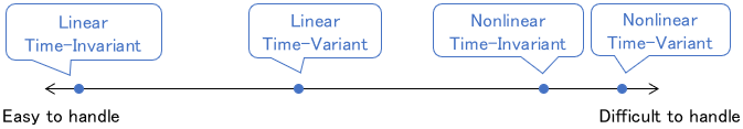
Time-Variant and Time-Invariant Systems
Linear and nonlinear systems are further divided into time-variant and time-invariant systems according to the form of the coefficients.
Specifically, systems whose coefficients are all constants are called time-invariant systems, while systems whose coefficients are time-dependent are called time-variant systems.
$$ \begin{alignat}{5} a_2 \ddot{y} &\ +\ a_1 \dot{y} & &\ +\ a_0 y &&\ =\ b_1 \dot{u} & &\ +\ b_0 u : & &\quad \textbf{Time-Invariant} \\ a_2 \ddot{y} &\ +\ \color{red}{a_1(t)} \dot{y} & &\ +\ a_0 y & &\ =\ b_1 \dot{u} & &\ +\ b_0 u : & &\quad \textbf{Time-Variant}\end{alignat} $$
Time-invariant systems are easier to handle than time-variant systems. Therefore, to distinguish them, they are sometimes called “Linear Time-Variant (LTV) systems” and “Linear Time-Invariant (LTI) systems,“ respectively.
On the other hand, since nonlinear systems are complex, the ease of handling does not change much, regardless of whether they are time-variant or time-invariant. Therefore, it is not common to distinguish them as “Nonlinear Time-Variant systems” or “Nonlinear Time-Invariant systems.”
The following figure shows the ease of use of each group.
Example of Linear Time-Invariant System
As an example, consider the following mechanical system.
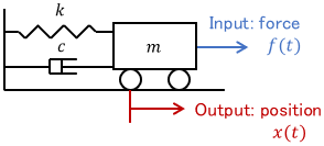
This system can be modeled as a linear time-invariant system as follows:
$$ m\ddot{x} + c\dot{x} + kx = f $$
As mentioned above, linear time-invariant systems are the easiest to deal with, so this is what is targeted at first in modeling. Therefore, in practice, most linear systems become time-invariant. Also, note that most systems dealt with in classical control are linear time-invariant.
Examples of Linear Time-Variant Systems
As explained earlier, most linear systems are modeled as time-invariant systems. So linear time-variant systems do not appear very often. In this section, situations in which linear time-variant systems can be used will be explained.
Note: The explanation goes into great detail, so those who just want to know the difference between linear and nonlinear systems may skip this section.
Examples of Linear Time-Variant Plant (rarely used)
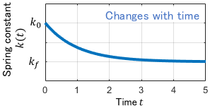
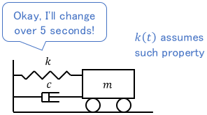
Let’s consider again the mechanical system we saw earlier.
Let’s also assume that as the system operates, the spring gradually warms up, and the spring constant $k$ changes accordingly from the initial value $k_0$ to $k_f$. The model for this system can be expressed as a linear time-variant system. For example
$$ \begin{align} \text{Model of Mechanical System:} & \quad m\ddot{x} + c\dot{x} + \color{red}{k(t)}x = f \\[3pt] \text{Model of Spring Constant:} & \quad \color{red}{k(t)} = (k_0 – k_f) e^{-t} + k_f \end{align}$$
Note: The above equation is just an example, so you only need to understand the concept here (the same applies hereafter).
The spring constant is modeled as a function of time, $k(t)$, so that it changes as time goes by (roughly over 5 seconds). Like this, changes in physical variables are sometimes modeled in a simplified manner as a function of time.
Note, however, that this is not a model that reflects the intrinsic nature of the plant. In fact, the spring constant is not essentially dependent on time but on the temperature of the spring, right?
Therefore, if the operating conditions (e.g., the surrounding temperature) change, the system properties will also change, and the above model will no longer be usable.
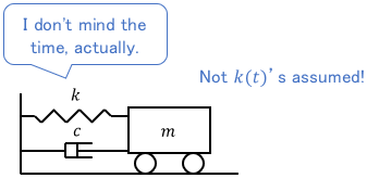
In this case, it becomes a more essential model if the spring constant is modeled as a function of temperature, $k(\theta)$.
$$ \begin{align} \text{Model of Mechanical System:} & \quad m\ddot{x} + c\dot{x} + k(\theta)x = f \\[3pt] \text{Model of Spring Constant:} & \quad k(\theta) = a_1 \theta + a_0 \end{align}$$
In this case, however, another model for the temperature change is required, which makes the overall equation more numerous and complex.
Thus, each of these models has advantages and disadvantages. Therefore, we need to decide which to use on a case-by-case basis. That is where the designer’s skill comes into play. But basically, we can assume that physical variables are rarely a function of time.
Example of Linear Time-Variant Controller (sometimes used)
On the other hand, since a person designs controllers, it is sometimes effective to make the control coefficients a function of time (i.e. make the controller a linear time-variant system).
For example, this is the case when the control is gradually enabled or disabled. As an example, consider the following simple proportional control system:
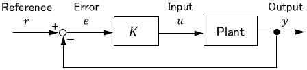
where $K$ is a constant control gain and the plant is a linear system. Let’s suppose the system goes wild immediately after the control starts, and that is problematic.
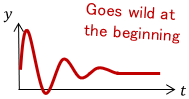
The cause of the problem seems to be that the control is turned on suddenly. Therefore, consider activating the control gradually. We can achieve this by applying the following time-variant coefficient $w(t)$ to the controller:
$$w(t) = 1 – e^{-t}$$
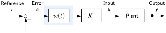
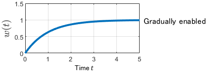
The control is gradually enabled by $w(t)$ over about 5 seconds. In this case, the controller can be interpreted as a linear time-variant system with input $e$ and output $u$. Of course, the entire system, including the controller and the plant, is also a linear time-variant system.
Note: This can also be interpreted as a control tuning technique called “gain scheduling.”
Example of Nonlinear System
An example of a simple nonlinear system is a pendulum.
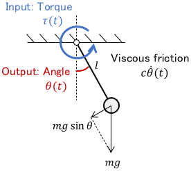
This system can be described by the following nonlinear equation of motion.
$$ml^2 \ddot{\theta} + c \dot{\theta} + mgl \ubg{ \sin \theta}{\text{Nonlinear}} = \tau$$
By the way, this is a time-invariant system since the coefficients are all constants.
As mentioned earlier, nonlinear systems are difficult to find exact solutions for, so some ingenuity is required to control them. In nonlinear control theory, the following approach is often taken:
- Finding a solution by brute force with a computer (e.g., numerical calculation)
- Forcing the controlled variable to converge to a certain value even if the exact solution is unknown (e.g., control using Lyapunov functions).
It is also common to approximate a nonlinear system to a usable linear system using methods such as the Taylor series approximation*. This reduces the model’s accuracy but provides an exact solution and allows linear control theories to be applied.
$$\begin{gather} \text{Approximating to }\sin \theta \approx \theta, \\[5pt] ml^2 \ddot{\theta}+ c \dot{\theta} + mgl \theta = \tau \quad \color{green}{\text{It’s now linear!}}\end{gather}$$
*For more details on the Taylor series approximation, please see this page:

- A linear system is one whose mathematical model is expressed only in terms of “coefficient × input/output(s derivative),” while other systems are nonlinear systems.
- A time-invariant system is one whose coefficients are all constants. A time-variant system is one whose coefficients are time-dependent.
- Linear systems are easy to handle. Nonlinear systems are more difficult to handle.
- Time-invariant systems are easy to handle. Time-variant systems are more difficult to handle.
Comments