This page explains the use, advantages, and formulas of the Laplace transform and the inverse Laplace transform. We present the Laplace transform table and a simple way to memorize it.
- Laplace transform is a type of variable transformation.
- It simplifies the handling of differential equations and frequency analysis.
- Since Laplace transform formula is complex, the Laplace transforms that are frequently applied in practice are usually memorized.
Laplace Transform: An Overview
What is Laplace Transform?
Laplace transform— a tool for analyzing linear differential equations, is a type of variable transformation.
Real-world phenomena are represented by differential equations in various fields of physics, for instance, the equation of motion is expressed by a differential equation.
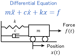
These differential equations are solved to extract physical significance from mathematical equations.
However, differential equations are complex and troublesome to handle. The Laplace transform is a mathematical technique developed to handle differential equations easily by manual calculation.
Terminologies and Mathematical Expressions
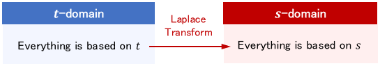
The basic variable in differential equations is time $t$. This time-based world is called $t$-domain (or time domain).
Laplace transform converts $t$ variable into $s$ variable and solves equations based on $s$. This $s$-based world is called $s$-domain (or frequency domain).
We convert a basic variable, thereby the expression in the formula will be naturally different. For example, $1$ in $t$-domain is represented by $\frac{1}{s}$ in s-domain.
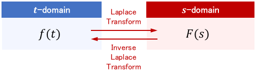
To further illustrate this, let us denote the representation of a function $f(t)$ in $s$-domain as $F(s)$. This $F(s)$ is called the “Laplace transform of $f(t)$.”
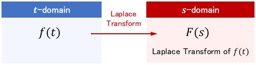
The operation of Laplace transforming $f(t)$ is represented as follows:
$$\mathcal{L} \big[ f(t)\big] = F(s)\quad \text{or} \quad f(t)\xrightarrow{\ \mathcal{L}\ }F(s)$$
Note: The first notation is often used in practice; we prefer second notation on this page for easy understanding.
Conversely, a variable transformation from $s$-domain to $t$-domain is called inverse Laplace transform.
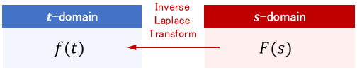
The operation of inverse Laplace transforming $F(s)$ is expressed as follows:
$$\mathcal{L}^{-1} \big[ F(s)\big] = f(t)\quad \text{or} \quad F(s)\xrightarrow{\mathcal{L}^{-1}}f(t)$$
Note that we are just looking at the same thing from different perspectives since both Laplace transform and inverse Laplace transform are just variable transforms.
Advantages and Uses of the Laplace Transform
Prior to perform Laplace transform, let’s first get a better picture of its advantages and uses to form a strong foundation for learning.
Advantage 1: Differential equations are easily evaluated by manual calculations
Laplace transform allows manual calculations of complex differential equations.
Specifically, “differentiate by time $t$” in $t$-domain turns into “multiply by $s$” in $s$-domain. Wow! A differentiation turns into a multiplication!
For example, consider the following differential equation:
$$\ddot{y}(t) + 2\dot{y}(t) + 3y(t) = 4\dot{x}(t) + 5x(t); \quad y(0)=\dot{y}(0)=0$$
It looks tedious to solve this because of the derivatives on both sides! Let us represent this equation in $s$-domain using Laplace transform.
$$s^2Y(s) + 2sY(s) + 3Y(s) = 4sX(s) + 5X(s)$$
where $X(s)$ and $Y(s)$ are the Laplace transforms of $x(t)$ and $y(t)$, respectively. In $s$-domain, there are no derivatives in the equation at all, and instead $s$ is multiplied to the functions as per respective number of derivatives.
As derivative is gone, solving this equation for $Y(s)$ is super easy.
$$Y(s) = \frac{4s+5}{s^2 + 2s + 3}X(s)$$
The solution $y(t)$ can be obtained by the inverse Laplace transform of $Y(s)$ (specific method is explained in further section).
Hence, the basic use of the Laplace transform is to first Laplace transform the problem, process the problem in $s$-domain, where the calculation is easy, and then transform the obtained solution to $t$-domain.
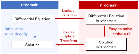
At this point, just keep in mind the above figure and the concept of derivatives turning into multiplication.
Advantage 2: High compatibility with frequency analysis
Uh-huh. So what is $s$ after all? I know $t$ represents time, but does $s$ mean something like that?
Although not as intuitive as $t$, if we interpret $f(t)$ as a kind of signal that changes from time to time, $s$ is known to be a parameter with a very close relation to its signal frequency.
This is because Laplace transform is mathematically similar to the Fourier transform—converting time $t$ to frequency.
Thus, in simple words, when we solve a differential equation using the Laplace transform, we can obtain not only the solution but also its frequency response.
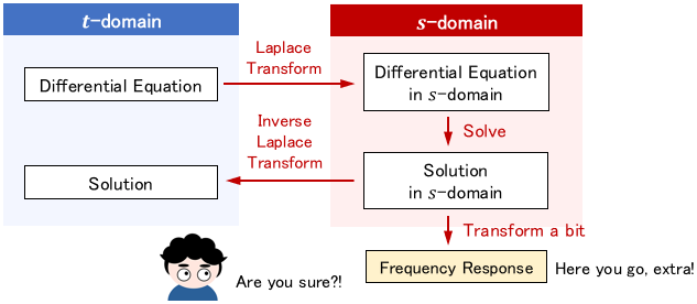
This virtue is useful in various engineering fields— especially frequency analysis in control engineering.
Definition of Laplace and inverse Laplace transforms
Let’s learn how to perform the Laplace and inverse Laplace transforms.
First, the Laplace transform $F(s)$ of function $f(t)$ is computed by the following equation. (This is the definition of the Laplace transform.)
$$F(s) = \int ^\infty _0 f(t)e^{-st}dt$$
Also, the inverse Laplace transform $f(t)$ of $F(s)$ is computed as follows
$$f(t) = \frac{1}{2\pi j}\int ^{c+j\infty} _{c-j\infty} F(s)e^{st}ds,\quad \text{where }\ c>0$$
Wow, that looks like a hassle…
You might think so. In fact, these can be calculated manually, but it is indeed tedious job.
Here comes a way! In the linear differential equations, the function $f(t)$ that appear in practice are limited.
Therefore, once you remember the function $f(t)$ and the corresponding $F(s)$ that often appear, you can do the transformations without using the above formulas. So, no worry!
Laplace Transforms of Frequently Appeared Functions
To avoid lengthy and tedious calculations, let’s look at the frequently used conversion formulas. We have only a few, so make sure you note them down!
Powers of Time
The first thing to keep in mind is the following conversion formula.
$$t^n\ \xrightarrow{\ \mathcal{L}\ }\ \frac{n!}{s^{n+1}}$$
Substituting $n=0,1,2$ into the above yields the following relation, which comes up particularly often.
$$1\ \xrightarrow{\ \mathcal{L}\ }\ \frac{1}{s}$$
$$ t\ \xrightarrow{\ \mathcal{L}\ }\ \frac{1}{s^2}$$
$$ t^2\ \xrightarrow{\ \mathcal{L}\ }\ \frac{2}{s^3}$$
We see that $1$ and $t$, which are basic elements in $t$-domain, are represented this way in $s$-domain.
Trigonometric Functions
We all know that sine and cosine functions are commonly practiced. The Laplace transform of both functions is expressed as follows:
$$\sin\omega t\ \xrightarrow{\ \mathcal{L}\ }\ \frac{\omega}{s^2+\omega ^2}$$
$$\cos\omega t\ \xrightarrow{\ \mathcal{L}\ }\ \frac{s}{s^2+\omega ^2}$$
Keep in mind that every formula can also be used as an inverse Laplace transform formula by reversing the arrow.
Basic Properties of Laplace and Inverse Laplace Transforms
Let’s explore more difficult problems where above functions appear in a slightly more complex form e.g., added together or differentiated.
To deal with the complexity of functions, let’s look at some useful properties of Laplace transform.
Linearity
What is Linearity?
Consider F(s) and G(s) as the Laplace transforms of the functions f(t) and g(t), respectively. The following relation holds for the sum of these functions.
$$f(t)+g(t) \ \xrightarrow{\ \mathcal{L}\ }\ F(s)+G(s)$$
Also, Laplace transform holds function multiplied with a constant, for instance, the equation is as follows:
$$af(t) \ \xrightarrow{\ \mathcal{L}\ }\ aF(s)$$
where $a$ is a constant. Combining the above yields the following relation.
$$af(t)+bg(t) \ \xrightarrow{\ \mathcal{L}\ }\ aF(s)+bG(s)$$
where $a$ and $b$ are constants. Simply put, the relation of functions with constants (addition/multiplication) remains the same in the transformation. This property is called linearity.
To note, the inverse Laplace transform also follows linearity. In other words, the relation holds even if the above arrows are reversed.
Example
Using linearity and the transformation formula from earlier, let’s find the Laplace transform of $2+3t+5x(t)$.
$$\begin{gather}\color{green}{\text{Formula to use:}}\quad \color{green}{1\ \xrightarrow{\ \mathcal{L}\ }\ \frac{1}{s}\quad \text{and} \quad t\ \xrightarrow{\ \mathcal{L}\ }\ \frac{1}{s^2}}\\[7pt] 2+3t+5x(t) \ \xrightarrow{\ \mathcal{L}\ }\ \frac{2}{s} + \frac{3}{s^2}+5X(s)\end{gather}$$
where $X(s)$ is the Laplace transform of $x(t)$. Like this, when a function is not explicitly defined in equation, you can just define the Laplace transform of it. So easy!
Pay Attention to Multiplication of Functions
Note that multiplication between functions does not hold linearity.
$$f(t)\cdot g(t) \ \xrightarrow{\ \mathcal{L}\ }\ F(s)\cdot G(s) \quad \color{red}{\text{does not hold!!}}$$
We will encounter such multiplication relations in practice. In such cases, the expression is transformed into addition using partial fraction decomposition.
Note: For more details on how to do partial fraction decomposition, please see this page:

Time Derivative
Laplace Transform of Time Derivative
The Laplace transform of the time derivative $\dot{f}(t)$ of the function $f(t)$ is
$$\dot{f}(t) \ \xrightarrow{\ \mathcal{L}\ }\ sF(s) – f(0)$$
where $f(0)$ is the initial value of $f(t)$ at $t=0$. In $s$-domain, the time differentiation is completely absent, and instead, the multiplication of $s$ variable and $F(s)$ appears. This property is tied to the greatest advantage of the Laplace transform.
In particular, if $f(0)=0$, the differentiation becomes a product of $s$ variable, as shown below:
$$\dot{f}(t) \ \xrightarrow{\ \mathcal{L}\ }\ sF(s) $$
Further, by differentiating the above formula, formulas for second-order and higher derivatives can also be obtained.
$$\begin{array}{lll}\ddot{f}(t) \ \xrightarrow{\ \mathcal{L}\ }& s\Big\{sF(s) – f(0)\Big\}-\dot{f}(0)&=s^2F(s)-sf(0)-\dot{f}(0) \\ \dddot{f}(t) \ \xrightarrow{\ \mathcal{L}\ }& s\Big\{s^2F(s)-sf(0)-\dot{f}(0)\Big\}-\ddot{f}(0)&=s^3F(s)-s^2f(0)-s\dot{f}(0)-\ddot{f}(0)\end{array}$$
Example
As an example, consider the Laplace transform of $\ddot{x}(t) + 2\dot{x}(t) + 3x(t) + 1 $.
$$\begin{align}\ddot{x}(t) + 2\dot{x}(t) + 3x(t) + 1 \ \xrightarrow{\ \mathcal{L}\ }\ &\Big\{s^2X(s)-sx(0)-\dot{x}(0)\Big\} + 2 \Big\{sX(s) – x(0)\Big\} + 3X(s) + \frac{1}{s} \\ &= \big( s^2 + 2s + 3\big)X(s) – \big( s+2\big)x(0) – \dot{x}(0) + \frac{1}{s}\end{align}$$
For $x(0)$ and $\dot{x}(0)$, you can simply assign the given initial values.
If $x(0)=\dot{x}(0)=0$, then the relation becomes as simple as multiplying $s$ by the number of derivatives.
$$\begin{align}\ddot{x}(t) + 2\dot{x}(t) + 3x(t) + 1 \ \xrightarrow{\ \mathcal{L}\ }\ &s^2 X(s) + 2sX(s) + 3X(s) + \frac{1}{s}\\ &= \big( s^2 + 2s + 3\big) X(s) + \frac{1}{s}\end{align}$$
Time Integration
Next, let’s explore the property of integration, which is the inverse of differentiation.
$$\int_0 ^t f(\tau)d\tau \ \xrightarrow{\ \mathcal{L}\ }\ \frac{1}{s}F(s)$$
It clearly shows that “divide by $s$” in $s$-domain corresponds to “integrate the function from time 0 to time $t$” in $t$-domain.
Since differentiation corresponds to the “multiply by $s$” in $s$-domain, it makes sense that integration corresponds to the “divide by $s$.”
This relation is ususally used to interpret formulas expressed in $s$-domain rather than direct conversion.
$$F(s)=\ubgd{sX(s)\vphantom{\frac{1}{s}}}{\text{Derivative}}{\text{of }x(t)}+\ubgd{\frac{1}{s}Y(s)}{\text{Integral}}{\text{of }y(t)}$$
Frequency Shifting
What is Frequency Shifting?
Finally, let’s look at a useful property—the frequency shifting theorem.
$$e^{at}f(t) \ \xrightarrow{\ \mathcal{L}\ }\ F(s-a)$$
where $a$ is a constant. The conversion shows that when function $f(t)$ is multiplied by $e^{at}$ in t-domain, the Laplace transform $F(s)$ is shifted by $a$ in s-domain.
This property is very useful because linear differential equations often involve $e^{at}$.
Example
By combining the frequency shifting with the Laplace transform formula described earlier, the applicability of the Laplace transform can be greatly expanded. Let’s look at the following combinations.
First, we calculate the Laplace transform of $e^{at}$.
$$\begin{gather}\color{green}{\text{Formula to use:}}\quad \color{green}{1\ \xrightarrow{\ \mathcal{L}\ }\ \frac{1}{s}}\\[7pt] e^{at}=e^{at}\cdot 1\ \xrightarrow{\ \mathcal{L}\ }\ \frac{1}{s-a}\end{gather}$$
The original transformation formula is shifted by $a$.
Generalizing for $t$ variable with frequency shifting, we obtain the following relation:
$$\begin{gather}\color{green}{\text{Formula to use:}}\quad \color{green}{t^n\ \xrightarrow{\ \mathcal{L}\ }\ \frac{n!}{s^{n+1}}}\\[7pt] t^n e^{at} \ \xrightarrow{\ \mathcal{L}\ }\ \frac{n!}{(s-a)^{n+1}}\end{gather}$$
Similarly, it applies on the trigonometric functions:
$$\begin{gather}\color{green}{\text{Formula to use:}}\quad \color{green}{\sin\omega t\ \xrightarrow{\ \mathcal{L}\ }\ \frac{\omega}{s^2+\omega ^2}}\\[7pt] e^{at}\sin\omega t\ \xrightarrow{\ \mathcal{L}\ }\ \frac{\omega}{(s-a)^2+\omega ^2}\end{gather}$$
$$\begin{gather}\color{green}{\text{Formula to use:}}\quad \color{green}{\cos\omega t\ \xrightarrow{\ \mathcal{L}\ }\ \frac{s}{s^2+\omega ^2}}\\[7pt] e^{at}\cos\omega t\ \xrightarrow{\ \mathcal{L}\ }\ \frac{s-a}{(s-a)^2+\omega ^2}\end{gather}$$
These relations are often used for inverse Laplace transforms.
Laplace Transform Table
From the above discussion, the list of commonly used Laplace transforms can be summarized as follows.
Basic Properties Table
| $t$-domain | $s$-domain | Remark |
|---|---|---|
| $af(t)+bg(t)$ | $aF(s)+bG(s)$ | Linearity |
| $\dot{f}(t)$ | $sF(s)-f(0)$ | Derivative |
| $\int_0 ^t f(\tau)d\tau$ | $\frac{1}{s}F(s)$ | Integral |
| $e^{at}f(t)$ | $F(s-a)$ | Frequency Shift |
Basic Transformation Table
| $t$-domain | $s$-domain | Remark | |
|---|---|---|---|
| #1 | $t^n$ | $\frac{n!}{s^{n+1}}$ | This is the base. |
| #2 | $1$ | $\frac{1}{s}$ | #1 with $n=0$ |
| #3 | $t$ | $\frac{1}{s^2}$ | #1 with $n=1$ |
| #4 | $t^2$ | $\frac{2}{s^3}$ | #1 with $n=2$ |
| #5 | $e^{at}$ | $\frac{1}{s-a}$ | #2 & Frequency Shift |
| #6 | $t^n e^{at}$ | $\frac{n!}{(s-a)^{n+1}}$ | #1 & Frequency Shift |
| $t$-domain | $s$-domain | Remark | |
|---|---|---|---|
| #1 | $\sin\omega t$ | $\frac{\omega}{s^2+\omega ^2}$ | This is the base. |
| #2 | $\cos\omega t$ | $ \frac{s}{s^2+\omega ^2}$ | This is the base too. |
| #3 | $e^{at}\sin\omega t$ | $\frac{\omega}{(s-a)^2+\omega ^2}$ | #1 & Frequency Shift |
| #4 | $e^{at}\cos\omega t$ | $\frac{s-a}{(s-a)^2+\omega ^2}$ | #2 & Frequency Shift |
Note: Just remember the base transformation formulas, you will derive most of the transformations like a Pro!
Nevertheless, practice makes you perfect. We recommend to solve problems to keep them in mind rather than try to memorize them.
Note: Please refer to the page below to learn how to solve differential equations using Laplace transform through various examples.
- Laplace transform is a type of variable transformation.
- It simplifies the handling of differential equations and frequency analysis.
- Since Laplace transform formula is complex, the Laplace transforms that are frequently applied in practice are usually memorized.
Comments