There are different control methods in the world. So, it is not easy to get the whole picture of all the control methods. This page gives a brief introduction to the major control methods.
Classical Control
Since classical control can only handle linear systems, controllers are also linearly configured. The following are typical controllers.
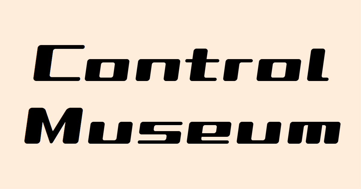
PID Control
PID control is a basic and simple control method consisting of proportional, integral, and derivative elements.
$$u(t) = \ubg{K_P\ e(t) \vphantom{K_I \int ^t _0 e(\tau) d\tau}}{\text{Proportional}} + \ubg{K_I \int ^t _0 e(\tau) d\tau}{\text{Integral}} + \ubg{K_D\ \dot{e}(t)\vphantom{K_I \int ^t _0 e(\tau) d\tau}}{\text{Derivative}}$$
Control performance is adjusted by tuning the gains $K_P$, $K_I$, and $K_D$. The tuning can be done theoretically using a mathematical model, but it is often done by trial and error while actually moving the plant (because it is easier).
The greatest advantage is its ease of use. Even those who know little about control engineering can easily achieve a performance of about 80 points. Although primitive, it is the most widely used controller in the world.
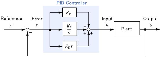
Control based on Frequency Analysis
This method considers what frequency characteristics a controller should have to realize desired frequency characteristics of the entire system.
The advantage is that it can handle more complex controllers than PID systems based on the theory.
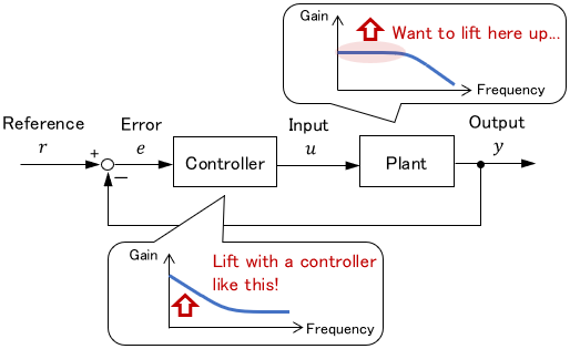
Root Locus
The root locus is a graphical representation of how the poles of a system change as a control gain is gradually increased. Based on the root locus, an appropriate control gain can be designed graphically.
Think of the pole as a convenient parameter that gives some idea of the system behavior without solving a mathematical model.
Since the movement of the poles on the root locus has some laws, the root locus can be drawn conveniently without actually calculating all poles.
One advantage of the root locus is that it provides a visual correspondence between the set gain and the behavior it produces. Although it was innovative and often used at the time, it is not used very often now that computer-based controller design has been developed.
Two-Degree-of-Freedom Control
Simply put, Two-Degree-of-Freedom (2-DOF) control is a combination of feedback control and feedforward control.
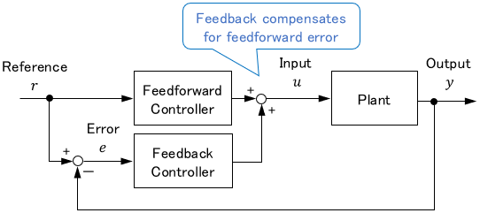
Standard feedback control is based only on the error $e$, while feedforward control is based only on the reference $r$. By combining the two, control based on two pieces of information, $e$ and $r$ (or $y$ and $r$), becomes possible. Thus it is called 2-DOF control.
The advantage of 2-DOF control is that it can combine feedback control’s high tracking accuracy with feedforward control’s fast response speed.
Note: For more details on feedback and feedforward control, please see this page:

Modern Control
Most modern control methods can handle both linear and nonlinear systems. All of the methods below have both linear and nonlinear theories. However, nonlinear methods are much more difficult to design and implement.
Note: For the difference between classical control and modern control, see this page:
Optimal Control
Optimal control is a method of calculating the optimal control input to achieve a control objective. The control objective is expressed by the following cost function $J$, and the optimal input that minimizes $J$ is then derived.
$$J= \ubg{\phi \bigl( x(t_f) \bigr)}{\text{Terminal cost}} + \ubg{\int ^{t_f} _{t_0} L\bigl(x(t), u(t)\bigr)dt}{\text{Running cost}} $$
The terminal cost reflects what we want the final state to be, and the running cost reflects how we want the state to reach the final state. Both are often set by the tracking error and the amount of control input. The designer’s skill is in how to reflect the control objectives in the cost function.
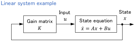
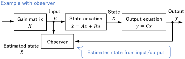
Usually, control inputs are derived in the form of state feedback.
If the state cannot be obtained directly by sensors, the state is often estimated by the observer or Kalman filter.
The greatest advantage of the optimal control is that it literally yields the optimal solution. This is a very powerful method unique to modern control, where all system characteristics are considered in the state equation.
The major types of linear optimal control are listed below:
- LQR control: The most basic optimal control that aims to bring the state to zero.
- LQI control: Optimal control that aims to bring the state to an arbitrary constant value.
- LQG control: Optimal control also considers the noise in the controlled plant. Simply put, it is a combination of LQR and Kalman filter.
Bang-Bang Control
Bang-Bang Control, also called on-off control, refers to control in which the control input takes either of two values only.
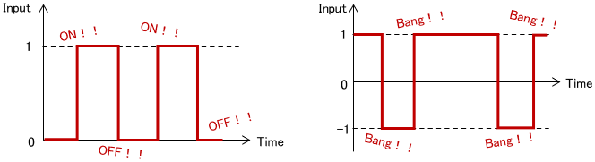
When a system can be controlled only by turning a switch on and off, it is essentially a bang-bang control. For example, some heaters control the temperature by turning on the operation when the temperature is lower than the set value and vice versa, which is bang-bang control.
The greatest advantage is that it can be realized with a cheap and simple configuration. On the other hand, the disadvantage is that the control input changes abruptly, which makes plant behavior unsmooth.
Also, there are cases where optimal control results in bang-bang control. A typical example is minimum time control. For example, consider moving a car from its current position to its destination.
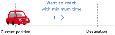
The control inputs are the gas pedal and brake operation, i.e. the acceleration of the car. In this case, the optimal control input that minimizes the time to reach the destination is the resulting bang-bang control.
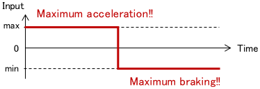
So it is best to first step on the accelerator to the maximum and then step on the brake to the maximum at a specific time. This makes intuitive sense.
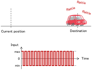
In reality, however, it is impossible to stop exactly at the destination, and chattering tends to occur. Therefore, some countermeasure is necessary.
Adaptive Control
Adaptive control is a method that automatically adjusts the parameters of controllers or mathematical models according to recent operating results.
Although optimal control is powerful, its performance is degraded if mathematical models have errors. Nevertheless, mathematical models always contain errors because the characteristics of real systems will vary with age and operating conditions. The advantage of adaptive control is that it can reduce such errors by automatically adjusting parameters.
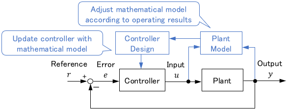
Adaptive control can be broadly classified into two types: Model Reference Adaptive Control (MRAC) and Self-Tuning Regulator.
MRAC is a method that adjusts controller parameters to compensate for errors in a model. It is also called the direct method.
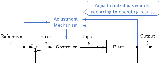
On the other hand, the self-tuning regulator adjusts the parameters of a model and redesigns the controller based on the adjusted model. It is also called the indirect method.
Robust Control
Robust control is a method that considers the range of uncertainty in a model to obtain stable results even in the worst-case scenario.
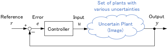
Before robust control, control engineering considered how to reduce modeling errors and create a nearly perfect model. Robust control can be interpreted as giving up on this and considering control that works even if the model is not perfect.
Of course, the advantage of robust control is that it is robust to uncertainties such as errors and disturbances. However, the design difficulty is greater because uncertainty must be considered in addition to the mathematical model.
Furthermore, we can say robust control is conservative control that always considers the worst case, so the control performance is lower than it should be if the model were perfect.
Typical robust control methods include H∞ control, μ-analysis, and methods with LMI. H∞ control is also used in classical control because it is highly compatible with the diagrammatic design methods of classical control.
Model Predictive Control
Model predictive control (or receding horizon control) is a method that continues to solve the optimal control problem from the present to a short time in the future during control, resulting in optimal feedback control.
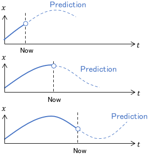
Other optimal control methods derive the optimal control law before control. On the other hand, model predictive control significantly differs because it continues to derive the optimal input during control.
Although it sounds like brute force, not having to exhaustively consider control laws in advance is quite a useful property in solving the problem.
The first advantage of model predictive control is that it can combine the advantages of feedback and feedforward controls. In addition, it is known to be quite practical, as it can respond to reference changes during control and can take into account input and state constraints.
Control based on Lyapunov Function
This method uses Lyapunov stability analysis to converge states or errors to zero. It is usually used to control nonlinear systems.
Lyapunov stability analysis is that for a system
$$\dot{x} = f(x),$$
if there is a Lyapunov function \(V(x)\) satisfying
$$\begin{align} V(x) &\succ 0 \\ \dot{V}(x) &\prec 0,\end{align}$$
then the system is asymptotically stable (i.e. \(\lim _{t\rightarrow \infty} x(t)= 0\)).
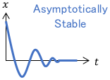
In other words, the variable $x$ is driven to 0 over time.
It is important to note that $x$ is not limited to the system’s state but can be anything. For example, if we set $x$ to be the error between a controlled variable and a reference, then the error will converge to zero over time, and tracking control can be achieved.
In such a case, the design flow looks like the following:
- Formulate the differential equation \(\dot{x} = f(x,u)\) for the error $x$
- Create a Lyapunov function candidate \(V(x)\succ 0\)
- Calculate \(\dot{V}(x)\) and \(\dot{x} = f(x,u)\) appears inside. Set the control input $u$ so that \(\dot{V}(x) \prec 0\) is satisfied.
The advantage of Lyapunov stability analysis is its very wide applicability since it can be applied regardless of linear or nonlinear systems.
On the other hand, the disadvantage is that a trial-and-error search for the Lyapunov function is required. Particularly in complex systems, one must be careful (and prepared) for the fact that Lyapunov functions tend to be unmanageably complex.
Sliding Mode Control
Sliding Mode Control is a control technique that confines the system behavior to a certain trajectory (or surface). It can be interpreted as an advanced version of Lyapunov function control. It is also usually used to control nonlinear systems.
First, for the system \(\dot{x} = f(x,u)\), the trajectory (or surface) is designed in the form of the following differential equation:
$$S(x)=0$$
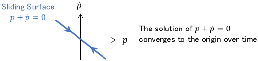
The surface by $S(x)$ in the state space is called the sliding surface. For example, for the following state $x$, the sliding surface can be set as follows:
$$ x = \left[ \begin{array} {c} p\\ \dot{p} \end{array} \right]$$
$$S(x) = \left[ \begin{array} {c c} 1 & 1 \end{array} \right]\left[ \begin{array} {c} p\\ \dot{p} \end{array} \right] = p + \dot{p} = 0$$
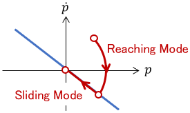
Now we set the Lyapunov function \(V(S)\) for \(S(x)\) and set the control input u so that it satisfies \(V(S) \succ 0\) and \( \dot{V}(S) \prec 0\). Then the system behavior is confined to the sliding surface \(S(x)=0\).
The system behavior in state space is such that the state first goes to the sliding surface (reaching mode) and then “slides” on the sliding surface (sliding mode).
The advantage of sliding mode control is that it is robust against modeling errors and disturbances. However, chattering tends to occur around the sliding surface, so some countermeasures are required.
Note: In addition to the above method using the Lyapunov function, various other methods have been proposed to confine the system behavior to the sliding surface.
Other Control Methods
Let me now introduce some control methods that are not included in the basic philosophy of control engineering, which is to design controllers based on a mathematical model of the plant.
Sequence Control
Sequence Control is a simple control method based on the ON/OFF of switches. Since it is not a control of physical variables based on mathematical models, it is not usually included in the framework of control engineering.
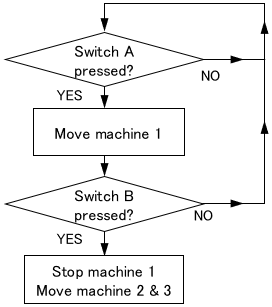
The control methods we have seen so far were intended to accurately control individual systems. On the other hand, sequence control is used to control the flow of operations (i.e. sequence) between systems as follows.
- Switch A is pressed
- Machine 1 moves.
- When machine 1 finishes its work, switch B is pressed
- Machine 1 stops, machines 2 and 3 start
This can be interpreted as a method based on the so-called IF-THEN rule.
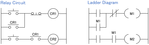
Initially, these sequences were realized with analog relay circuits. Since the 1970s, PLCs (programmable logic controllers), which allow sequences to be programmed on software, have been popular and widely used.
The advantage of PLCs is that they do not require advanced control or programming knowledge, since they are programmed by simply creating a ladder diagram, similar to an analog relay circuit, in software.
Sequence control is widely used in various applications, including automatic doors, conveyor belts, and overhead cranes.
Fuzzy Control
Fuzzy control is a control method that aims to reproduce rough knowledge of human beings, such as “In this case, if I operate the machine in this way, it will operate in a good way!”
First, human knowledge is compiled into rules. In the case of driving a car, the rules may look like this:
- IF the speed is “low”AND the car distance is “short,” THEN maintain the speed.
- IF the speed is “low”AND the distance is “long,” THEN increase the speed.
- IF the speed is “high” AND the distance is “short,” THEN decrease the speed.
- IF the speed is “high” AND the distance is “long,” THEN maintain the speed.
Then, a membership function is defined to link the “degree” of each state with a physical quantity.
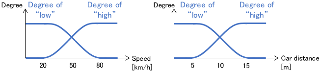
During control, the membership function calculates the degree of conformance to each rule for the current state.
Rule conformance for the current state
- IF the speed is “low” AND the car distance is “short,” THEN maintain the speed: 30%
- IF the speed is “low” AND the distance is “long,” THEN increase the speed: 10%
- IF the speed is “high” AND the distance is “short,” THEN decrease the speed: 80%
- IF the speed is “high” AND the distance is “long,” THEN maintain the speed: 20%
Finally, the control input is determined according to the conformance level as follows:
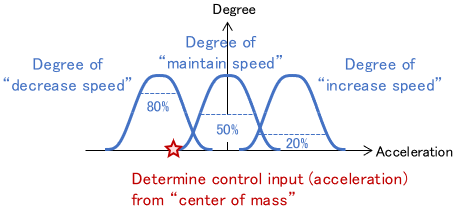
Note: The above is just an example, and various other fuzzy control laws have been proposed.
One advantage of fuzzy control is that it can utilize human empirical rules for control that are not based on mathematical models. It is truly a control method that reproduces “fuzzy” human knowledge.
Reinforcement Learning
Reinforcement Learning is a method of having a computer learn optimal control laws through trial and error.
The greatest advantage of this method is that it can learn even without a model of the plant because it is based on trial-and-error.
Since a huge number of trial-and-error operations are required in most cases, trial-and-error is mostly performed at high speed on a simulation. Therefore, it is suitable for objects whose behavior can be simulated quickly and completely on a computer, such as games and planning problems.
On the other hand, its application to real systems such as robots and cars is still limited. For example, it takes several months to perform trial-and-error on a real robot. Also, the controller in the early stages of learning is almost always in a runaway state, which is very dangerous.
If you train the robot quickly and safely by simulation, the training results will not be applicable in the real world because simulation models always have errors. Even if we can prepare an error-free model, we can use optimal control in such a case, making reinforcement learning meaningless. (since it is optimal, it will always produce a better solution than reinforcement learning). Thus, there are still challenges in applying reinforcement learning to real systems.
However, it is a field that continues to make remarkable progress thanks to recent developments in computational technology. Therefore, new and more practical methods may be developed in the future.
Comments