
Control engineering can be broadly divided into two fields: classical control and modern control. This page explains the differences between them and the advantages of each field.
| Classical Control | Modern Control | |
|---|---|---|
| Main calculation method | Manual calculation | Computer calculation |
| Supported input/output | Single input & single output only | Multiple input & multiple output |
| Supported system | Linear time-invariant system only | Almost any system |
| Variable domain | $s$-domain (frequency domain) | $t$-domain (time domain) |
| System representation | Transfer function | State equation |
- Basically, modern control has more capabilities and higher performance.
- However, classical control has its strengths, such as frequency analysis and stability margin analysis.
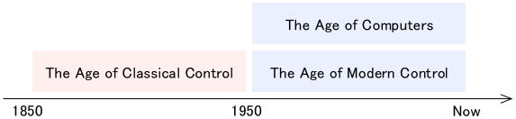
Origin of the Terms
The terms “classic” and “modern” were derived from history.
Classical control has been actively researched since around 1850 and was almost in its current form around 1950. On the other hand, modern control has been actively studied since about 1950 and continues to evolve.
Based on this history, they are distinguished by the terms “classic” and “modern,” respectively.
The key to considering the two is whether or not they assume the existence of computers. We can interpret that classical control assumes manual calculations and modern control assumes computer calculations.
Differences in Target Systems
Difference in Number of Input/Output
Classical Control
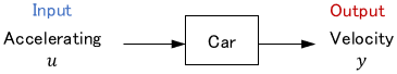
Classical control can only handle single-input and single-output (SISO) systems.
Modern Control
Modern control, on the other hand, has no limit to the number of inputs and outputs. In other words, it can handle multiple-input and multiple-output (MIMO) systems.
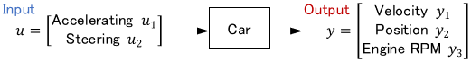
When classical control handles a MIMO system, we must reduce the number of signals to convert the system to SISO. On the other hand, modern control can handle the plant as it is.
Difference in Mathematical Model Structure
Classical Control
Classical control can only handle systems whose mathematical models are linear and time-invariant (with a few exceptions). Such systems are called “Linear Time-Invariant (LTI) systems.”
Simply put, an LTI system is a system whose mathematical model is expressed only in terms of “constant × input/output(s derivative),” like the following equation.
$$a_2 \ddot{y} + a_1 \dot y + a_0 y = b_1 \dot u + b_0 u$$
Modern Control
On the other hand, modern control can handle various systems, whether linear, nonlinear, time-variant, or time-invariant. You can consider that it can handle almost any system.
Of course, the more complex the system is, the more difficult it is to handle. Modern control solves this mainly through computer calculations.
Note: For more information on the difference between linear, nonlinear, time-variant, and time-invariant systems, please see this page:

Differences in System Representations
Difference in Base Variables
Modern Control
Let’s look at modern control first, as it will be easier to understand.
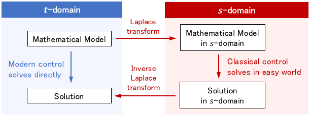
In modern control, mathematical models are based on time $t$. This time-based world is called the $t$-domain (or time domain). The good thing is that it is intuitive.
However, since most of the mathematical models are differential equations, in most cases, it is difficult to solve them as they are.

Classical Control
Classical control, on the other hand, uses a variable transformation called the Laplace transform to transform time $t$ into a variable $s$. It then handles the mathematical model based on the $s$.
This $s$-based world is called the $s$-domain (or frequency domain). It is known that in the $s$-domain, it is effortless to solve differential equations by hand.

As shown in the figure below, the basic idea is to first convert the problem to the $s$-domain, deal with it in the world of easy calculations, and then return the obtained answer to the $t$-domain.
Note: For more details on the Laplace transform, please see this page:
Difference in Mathematical Model Representations
The base variables are different. For this reason, the mathematical model expressions are naturally different between classical and modern control.
Let’s look at the differences using the following mechanical system as an example.
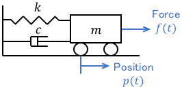
where $p(t)$ is the position of the cart, $f(t)$ is the force acting on the cart, $m$ is the mass of the cart, $k$ is the spring constant, and $c$ is the viscous friction coefficient. The characteristic of this system is expressed by the equation of motion as follows:
$$m\ddot{p} + c \dot{p} + kp = f$$
Classical Control
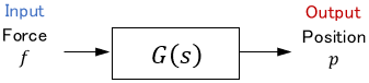
In classical control, calculations are performed in the $s$-domain, so mathematical models are expressed in terms of $s$. This s-based mathematical model is called the transfer function.
$$\text{Transfer function example:}\ \ G(s) = \frac{b_1 s + b_0}{s^2 + a_1 s + a_0}$$
where $a_∗$ and $b_∗$ are constants. The mechanical system described earlier can be expressed by the transfer function as follows:
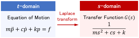
As shown in the figure, the transfer function is the Laplace transform of the mathematical model expressed in the $t$-domain. In a block diagram, it is represented as shown below:
Note: For more details on the transfer function, please see this page:
Modern Control
On the other hand, modern control uses vectors and matrices to express a system as a first-order simultaneous differential equation based on time $t$. This equation is called the state equation.
$$\text{State equation example:}\ \ \dot{x} = Ax + Bu $$
where $x$ is the state vector, $u$ is the input vector, and $A$ and $B$ are matrices. The mechanical system described earlier can be expressed by the state equation as follows:
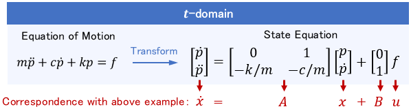
While transfer functions consider only the relation between input and output, state equations take into account all variables that make up a mathematical model as the “state” of the system.
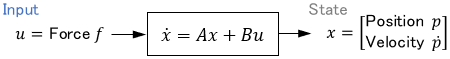
In the example above, not only the position $p$, but also the velocity $\dot{p}$ are considered in the state $x$. This is a simple example, but the more complex the system, the more states are considered.
However, this alone does not tell us which information in state $x$ can be taken out as output. Therefore, an output equation is used to express the relation between state and output.
$$\text{Output equation example:}\ \ y = Cx $$
where $y$ is the output vector and $C$ is a matrix. For instance, in the mechanical system described earlier, if only the position $p$ can be obtained by the sensor (i.e. taken as output), the output equation is represented as follows:
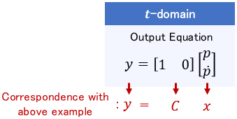
Like this, the output equation usually represents which states can actually be obtained (e.g., by a sensor).
In summary, a system in modern control is represented by the following block diagram, which combines the state equation and the output equation.
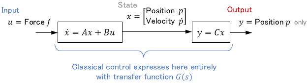
This way of representing a system is called a state-space representation.
In classical control, the transfer function only briefly represents the relation between input and output. In contrast, the state equation in modern control considers everything inside the system.
Difference in Advantages
Modern Control
As described above, modern control can handle a wide variety of systems, and it considers all system internals. Therefore, it is easier to achieve higher performance than classical control.
Particularly, optimal control, which calculates the optimal control input for the control objective, is a powerful control method representing modern control.
Classical Control
Classical control, on the other hand, can only handle SISO systems and only considers input-output relation. So it is not as powerful as modern control in most cases.
However, classical control has unique strengths not found in modern control, such as frequency analysis and stability margin analysis.
Frequency Analysis
Frequency analysis is a technique for analyzing how a system responds to various frequency signal components. (Think of frequency as how fast a signal changes).
It allows us to obtain information about a target system, such as “particularly sensitive to this frequency” or “less responsive to frequencies above here.”
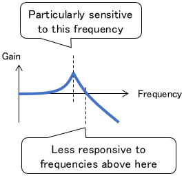
Frequency analysis is a specialty of classical control since the Laplace transform is compatible with frequency analysis.
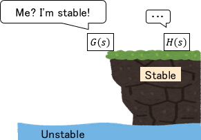
Stability Margin Analysis
Stability margin analysis is a method that analyzes the degree of stability of a system, such as whether the system is stable with margin or just barely stable.
This is very useful because it is problematic if a system is just barely stable in practical use.
Difference in Applications
Modern Control
Modern control is often used for systems whose mathematical models can be derived accurately.
For example, in mechanical systems, modern control is often applied to robots, carts, drones, etc., whose characteristics can be expressed by equations of motion.
In electrical systems, it is often applied to regulator circuits, motor circuits, etc., whose characteristics can be expressed by differential equations.
Modern control is often used for advanced control objectives such as minimizing motion errors or maximizing energy efficiency.
Classical Control
Classical control is often used for systems whose frequency response is particularly important.
For example, in mechanical systems, classical control is often used for vibration suppression control where the vibration frequency is important.
In electrical systems, it is used to design filter circuits that cut off specific frequency inputs.

Classical control is also often used when the user does not know the exact mathematical model but wants to run the system with a good performance quickly. This is exactly the purpose of control in the era when classical control was first used.

For example, PID control can easily produce good performance through trial-and-error parameter tuning, even if the system model is completely unknown. It is so widely used and practical that it is said that 80% of controllers in the world are PID.
This page explained the differences between them and the advantages of each field. To conclude, a summary is shown here.
| Classical Control | Modern Control | |
|---|---|---|
| Main calculation method | Manual calculation | Computer calculation |
| Supported input/output | Single input & single output only | Multiple input & multiple output |
| Supported system | Linear time-invariant system only | Almost any system |
| Variable domain | $s$-domain (frequency domain) | $t$-domain (time domain) |
| System representation | Transfer function | State equation |
- Basically, modern control has more capabilities and higher performance.
- However, classical control has its strengths, such as frequency analysis and stability margin analysis.
Comments