
The following functional representation is called Taylor series.
$$f(x) = f(a) + f^{\prime}(a)(x-a) + \frac{f^{\prime \prime}(a)}{2!}(x-a)^2 + \frac{f^{\prime \prime \prime}(a)}{3!}(x-a)^3 + \cdots$$
..err… I don’t get it…
This formula may seem complicated, but once you grasp its meaning, you will accept its reasonable form. This page explains the concept, meaning, and uses of the Taylor series with examples.
- Taylor series is a polynomial representation of a function.
- It simplifies a function around a reference point.
- The key point is that at the reference point, all possible derivatives equate to the original function.
- To satisfy that, Taylor series formula shows a complicated form. But once you understand the meaning, it’s easy to remember!
Concept of Taylor Series
What is Taylor Series?
The expression of a function in a polynomial form is called Taylor series.
$$f(x) = k_0 + k_1 (x-a) + k_2 (x-a)^2 + k_3 (x-a)^3 + \cdots$$
where $k_0,k_1,\ldots$ and $a$ are constants. Expanding a function to the Taylor series is also termed as Taylor (series) expansion.
The above Taylor series is organized in $(x-a)$, but expanding it eventually leads the following simple polynomial expression.
$$f(x) = K_0 + K_1 x + K_2 x^2 + K_3 x^3 + \cdots$$
where \(K_0,K_1,\ldots\) are constants to denote the expansion result. For better clarification, the following discussion is based on the form with $(x-a)$.
Approximation with Taylor Polynomial
In practice, it is impossible to calculate an infinite number of series, so the calculation must be terminated at some point. In this case, the calculated part becomes an approximation of the function $f(x)$, and the remaining part becomes the approximation error (Remainder).
$$f(x) = \ubg{k_0 + k_1 (x-a) + k_2 (x-a)^2}{\large \text{Calculate only here}} +\ubg{k_3 (x-a)^3 + \cdots}{\large \text{Error}} $$
$$\text{Approximation: } f(x) \approx k_0 + k_1 (x-a) + k_2 (x-a)^2$$
The calculated part is called Taylor polynomial, and the approximation of a function in the Taylor polynomial is called the Taylor series approximation.
Naturally, for better approximation accuracy, more terms are considered. A Taylor polynomial with $n$ terms is called $n$-th order Taylor polynomial (or $n$-th order approximation).
| Order | Taylor polynomial | Function type |
|---|---|---|
| 0th-order | $f(x)\approx k_0$ | Constant |
| 1st-order | $f(x)\approx k_0 + k_1 (x-a)$ | Linear function |
| 2nd-order | $f(x)\approx k_0 + k_1 (x-a) + k_2 (x-a)^2$ | Quadratic function |
Concept of Coefficients
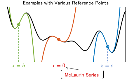
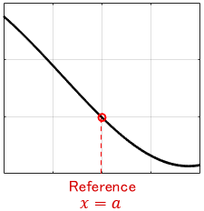
Now the key concern is how to choose the coefficients: \(k_0,k_1,\ldots\). In the Taylor series (approximation), the coefficients are determined to achieve the highest accuracy around a reference point $a$ on the $x$-axis.

More specifically, at the reference point $x=a$, the coefficients are determined to equate all possible derivatives to the original function.
As a result, we obtain the following complex Taylor series formula.
$$f(x) = \ubg{f(a)}{k_0} + \ubg{f^{\prime}(a)}{k_1} (x-a) + \ubg{\frac{f^{\prime \prime}(a)}{2!}}{k_2} (x-a)^2 + \ubg{\frac{f^{\prime \prime \prime}(a)}{3!}}{k_3} (x-a)^3 + \cdots$$
It looks complicated but easy to interpret if we consider that all factors except $(x-a)^k$ are coefficients. The factorial form of the coefficients is explained in detail later.
The approximation results varies along with the reference point. When the reference point should be explicit, we say, “Taylor series (approximation) around $x=a$.” In particular, Taylor series around $x=0$ is called the McLaurin series.
Uses and Examples of Taylor Series
Uh-huh. So, what can we use the Taylor series for?
Taylor series can simplify a function around a reference point, even though there may be a small error. Let’s look at some examples to understand the concepts and benefits intuitively.
Taylor Series of Exponential Function
Consider Taylor series of \(e^x\) around \(x=0\) (McLaughlin series of \(e^x\)) as a typical example for an exponential function.
$$e^x = 1 + \frac{x}{1!} + \frac{x^2}{2!} + \frac{x^3}{3!} + \frac{x^4}{4!} + \frac{x^5}{5!}+ \cdots$$
Let’s consider the Taylor series approximation of this. Increasing order yields the following:

Note: The red line represents the Taylor series approximation.
It’s a crude approximation at first, but as the order goes up, it fits the original function around \(x=0\).
Taylor Series of Sine Function
The Taylor series of the sine function around $x=0$ (McLaughlin series) is as follows:
$$\sin x = x – \frac{x^3}{3!} + \frac{x^5}{5!} – \frac{x^7}{7!} + \frac{x^9}{9!} – \cdots$$
The Taylor series consists of odd order terms only. Let’s consider the Taylor series approximation of this.

As before, the higher the order, the better the accuracy. In particular, the 1st-order approximation (i.e. linear approximation) of the sine function is often used in practice.

The reason is simple: we use the sine function frequently in many fields, but complex dealing. It would be nice if \(\sin x\) became just \(x\), wouldn’t it? The above figure shows that if we use the sine function only near \(x=0\), we can simplify it as \(\sin x \approx x\) with small error.
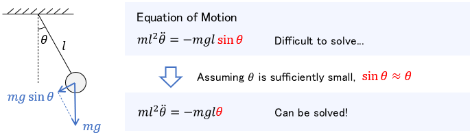
A major example is the equation of motion of a pendulum. It involves a sine function, which makes manual calculation difficult. However, if we assume that the pendulum’s angle is sufficiently small and apply the approximation \(\sin \theta \approx \theta\), the equation becomes simple to solve manually.
Thus, main use of Taylor series is to enable the computation of complex formulas by simplifying the function. In particular, 1st-order approximation (i.e. linear approximation) is often used for its simplicity. Any function looks like a straight line if you zoom in very much!
Let’s see what range of angles can be used for a linear approximation of the sine function. Here is the linear approximation graph with the range of small angles zoomed in. (For clarity, the horizontal axis unit is degree)

Of course, it depends on the application, but generally considered ±10° with little error.
Taylor Series of Cosine Function
The Taylor series of the cosine function around $x=0$ (McLaughlin series) is as follows:
$$\cos x = 1 – \frac{x^2}{2!} + \frac{x^4}{4!} – \frac{x^6}{6!} + \frac{x^8}{8!} – \cdots$$
The Taylor series consists of even order terms only. Let’s consider the Taylor series approximation of this.

The cosine function is lateral shift of the sine function, so we can interpreted it as the previous example with different reference point. However, the approximation accuracy looks different.
In particular, the linear approximation (i.e. 0th-order approximation) of the cosine function looks awful unlike the sine function.
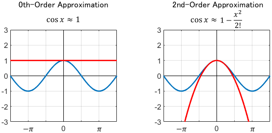
The 2nd-order approximation looks good, but it is rarely used. This is because a quadratic function is as complex as the cosine function and there is little advantage to approximate.
As described above, the accuracy of the Taylor series approximation depends on the function and the reference point. It is important to have a firm grasp of the function’s properties before using it.
Meaning of Taylor Series Formula
Now, let’s check insights into this complicated formula.
$$f(x) = f(a) + f^{\prime}(a)(x-a) + \frac{f^{\prime \prime}(a)}{2!}(x-a)^2 + \frac{f^{\prime \prime \prime}(a)}{3!}(x-a)^3 + \cdots$$
As you may have noticed, each term follows a law. The $n$-th term is expressed as
$$\ubgd{\frac{f^{(n)}(a)}{n!}}{\large \ \ \ \text{Just a}}{\large \text{coefficient}} (x-a)^n.$$
As mentioned earlier, the coefficients are determined to equate all possible derivatives to the original function. Let’s explore why each term has such form through Taylor series approximation of the following function.
To distinguish it from the original function \(f(x)\), we denote the approximated function as \(\tilde{f}(x)\).
$$f(x) \approx \tilde{f}(x)$$
Now, let’s look at the details of the Taylor series approximation by increasing the number of terms one by one.
0th-Order Approximation
First, consider the first term of the Taylor series.
$$\tilde{f}(x) = \ubg{f(a)}{\large \text{0th-order}} $$
It expresses the function with a constant. We use $f(a)$ that defines the value at the reference point $x=a$.

But it’s too simple to extract details, isn’t it? Let’s add more terms and improve the accuracy.
1st-Order Approximation
$$\tilde{f}(x) = f(a) + \ubg{f^{\prime}(a)(x-a)}{\large \text{1st-order}} $$
Herein, the 1st-order term is added, making it a linear function. This is the formula of a straight line with the same value and slope as the original function $f(x)$ at the reference point $x=a$. These properties are expressed as follows:
$$\begin{alignat}{2} &\text{Approximated function } &&\tilde{f}(a) = f(a) \\&\text{1st-order derivative } &&\tilde{f}^{\prime}(a) = f^{\prime}(a) \end{alignat}$$
Simply put, it’s the tangent line to $f(x)$ at the reference point!

Let’s interpret the equation form more intuitively. We can see that the additional 1st-order term works as follows.
- At $x=a$, no correction is made (due to no error in the 0th-order term $f(a)$).
- Away from $x=a$, the more correction is made based on the slope \(f^{\prime}(a)\)
$$\tilde{f}(x) = f(a) + \ubgd{f^{\prime}(a)(x-a)}{\large \text{Disappears at }x=a,}{\large \text{Corrects when } x \neq a} $$
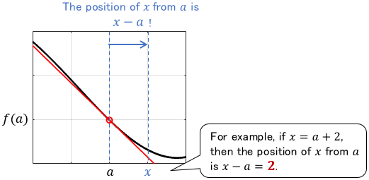
Thus, the Taylor series formula is based on $(x−a)$, which allows contribution from additional terms only when it needed.
$(x-a)$ represents “the position of $x$ as seen from $a$.” Therefore, the error can be corrected according to distance from the reference point $x=a$.
Nevertheless, it deviates, although this may be sufficient if $f(x)$ is only used in a very close neighborhood of $x=a$. Let’s add more terms to further compensate errors in the 1st-order approximation.
2nd-Order Approximation
$$\tilde{f}(x) = f(a) + f^{\prime}(a)(x-a) + \ubg{\frac{f^{\prime \prime}(a)}{2!}(x-a)^2}{\large \text{2nd-order}} $$

Now, it is a quadratic function, which is more accurate than the previous one. The 2nd-order term compensates errors in the 1st-order approximation. Let’s interpret this from the formula.
The problem with the 1st-order approximation is that it only represents a straight line with a constant slope. In fact, we need to bend the line a bit more to fit.
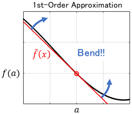
To bend the line, we require the slope change rate, i.e. 2nd-order derivative. Thanks to the 2nd-order term, we can derive the 2nd-order derivative of the approximated function \(\tilde{f}(x)\). Let’s calculate the derivatives.
$$\begin{alignat}{2} &\text{Approximated function }\ && \tilde{f}(x) = f(a) + f^{\prime}(a)(x-a) + \frac{f^{\prime \prime}(a)}{2!}(x-a)^2\\ &\text{1stst-order derivative }\ && \tilde{f}^{\prime}(x)= f^{\prime}(a) + f^{\prime \prime}(a)(x-a) \\[3pt] &\text{2nd-order derivative }\ &&\tilde{f}^{\prime \prime}(x)= f^{\prime \prime}(a)\end{alignat}$$
The 2nd-order derivative becomes \(f^{\prime \prime}(a)\). By substituting $x=a$ to the above equations, we find the following properties at the reference point.
$$\begin{alignat}{2}&\text{Approximated function } \ &&\tilde{f}(a) = f(a) \\[3pt] &\text{1st-order derivative }\ &&\tilde{f}^{\prime}(a)= f^{\prime}(a) \\[3pt] &\text{2nd-order derivative }\ && \tilde{f}^{\prime \prime}(a) = f^{\prime \prime}(a)\end{alignat}$$
Where, the approximated quadratic function \(\tilde{f}(x)\) shows the same value, slope, and slope change rate as the original function $f(x)$ at the reference point $x=a$.
To note, the 2nd-order term does not interfere with the other terms at the reference point $x=a$. This can be summarized as follows:
- At $x=a$, no correction is made to \(\tilde{f}(x)\) (due to no error in the 0th-order term $f(a)$).
- At $x=a$, no correction is made to \(\tilde{f}^{\prime}(x)\) either (in order not to change the slope \(f^{\prime}(a)\) created by the 1st-order term).
- Away from $x=a$, the more correction is made based on the slope change rate \(f^{\prime \prime}(a)\)
$$\begin{alignat}{2} &\text{Approximated function }\ && \tilde{f}(x) = f(a) + f^{\prime}(a)(x-a) + \ubgd{\frac{f^{\prime \prime}(a)}{2!}(x-a)^2}{\large \text{Disappears at }x=a,}{\large \text{Corrects when } x \neq a}\\ &\text{1st-order derivative } && \tilde{f}^{\prime}(x)= f^{\prime}(a) + \ubgd{f^{\prime \prime}(a)(x-a)}{\large \text{Disappears at }x=a,}{\large \text{Corrects when } x \neq a} \end{alignat}$$
The above outcomes are achieved because of the formula based on $(x-a)$. Thanks to this, all unnecessary terms disappear at $x=a$.
However, the accuracy is still degraded as we move away from the reference point. Let’s add the 3rd-order term to further compensate errors.
3rd-Order Approximation
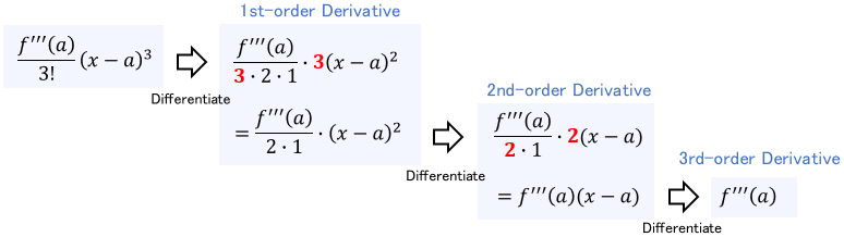
$$\tilde{f}(x) = f(a) + f^{\prime}(a)(x-a) + \frac{f^{\prime \prime}(a)}{2!}(x-a)^2 + \ubg{\frac{f^{\prime \prime \prime}(a)}{3!}(x-a)^3}{\large \text{3rd-order}} $$

Wow! We got precise fitting; it is a cubic function. Although the formula becomes long, the basic idea is the same as the 2nd-order approximation. Let’s get curious about a new discovery in the second half.
The limitation of the 2nd-order approximation is the constant slope change rate. So let’s consider the “change rate of the slope change rate,” i.e. 3rd-order derivative.
$$\begin{alignat}{2}&\text{Approximated function }\ && \tilde{f}(x) = f(a) + f^{\prime}(a)(x-a) + \frac{f^{\prime \prime}(a)}{2!}(x-a)^2 + \frac{f^{\prime \prime \prime}(a)}{3!}(x-a)^3 \\[1pt]&\text{1st-order derivative }\ && \tilde{f}^{\prime}(x) = f^{\prime}(a) + f^{\prime \prime}(a)(x-a) + \frac{f^{\prime \prime \prime}(a)}{2!}(x-a)^2 \\[3pt] &\text{2nd-order derivative }\ && \tilde{f}^{\prime \prime}(x) = f^{\prime \prime}(a) + f^{\prime \prime \prime}(a)(x-a) \\[6pt]&\text{3rd-order derivative }\ && \tilde{f}^{\prime \prime \prime}(x) = f^{\prime \prime \prime}(a) \end{alignat}$$
The 3rd-order derivative becomes \(f^{\prime \prime \prime}(a)\). By substituting $x=a$ to the above equations, we find the following properties at the reference point.
$$\begin{alignat}{2}&\text{Approximated function }\ && \tilde{f}(a) = f(a) \\[3pt]&\text{1st-order derivative }\ &&\tilde{f}^{\prime}(a)= f^{\prime}(a) \\[3pt]&\text{2nd-order derivative }\ && \tilde{f}^{\prime \prime}(a)= f^{\prime \prime}(a) \\[3pt]&\text{3rd-order derivative }\ && \tilde{f}^{\prime \prime \prime}(a)= f^{\prime \prime \prime}(a)\end{alignat}$$
Where, the approximated cubic function \(\tilde{f}(x)\) shows the same value, slope, slope change rate, and change rate of the slope change rate as the original function $f(x)$ at the reference point $x=a$.
As in the 2nd-order case, the expression based on $(x-a)$ ensures that the 3rd-order term does not interfere with the other terms at the reference point $x=a$.
What is new here—while differentiating \(\tilde{f}(x)\), the exponent of $(x-a)$ cancel out by the factorial. For example, when calculating the 3rd-order derivative of the 3rd-order term, the exponents cancel out one after the other, leaving only \(f^{\prime \prime \prime}(a)\) in the end.
That is why the mysterious exclamation marks are in the Taylor series!
nth-Order Approximation
Again, the equation is extended with the same idea. The nth-order approximation can be expressed as
$$f(x) = f(a) + f^{\prime}(a)(x-a) + \frac{f^{\prime \prime}(a)}{2!}(x-a)^2 + \cdots + \ubg{\frac{f^{(n)}(a)}{n!}(x-a)^n}{\large n\text{th-order}} $$
The idea so far is summarized as follows:
- Express the term based on \((x-a)^n\) to avoid interference with the other terms at the reference point $x=a$.
- Multiply it by \(\frac{1}{n!}\) to cancel out the coefficients while differentiated.
- Then the $n$th derivative becomes \(f^{(n)}(a)\), which means \(\tilde{f}^{(n)}(a) = f^{(n)}(a)\). In other words, at the reference point, the $n$th derivative becomes equal to the original function!
This is extended endlessly to form the Taylor series formula.
$$f(x) = f(a) + f^{\prime}(a)(x-a) + \frac{f^{\prime \prime}(a)}{2!}(x-a)^2 + \frac{f^{\prime \prime \prime}(a)}{3!}(x-a)^3 + \cdots$$
If the reference point is $a=0$, we obtain the McLaughlin series.
$$f(x) = f(0) + f^{\prime}(0)x + \frac{f^{\prime \prime}(0)}{2!}x^2 + \frac{f^{\prime \prime \prime}(0)}{3!}x^3 + \cdots $$
- Taylor series is a polynomial representation of a function.
- It simplifies a function around a reference point.
- The key point is that at the reference point, all possible derivatives equate to the original function.
- To satisfy that, Taylor series formula shows a complicated form. But once you understand the meaning, it’s easy to remember!
Comments