
This page introduces transfer functions of higher-order systems often encountered in practice, including the derivation process.
Higher-order systems often consist of several simple systems. For the basic concept of higher-order systems, please see this page:

Inverted Pendulum
First, consider an inverted pendulum as an example of two mechanical systems combined. Although there are many types of inverted pendulums, the one with a pendulum on a cart is often used as an example of mechanical control.

The input is the force $f(t)$ applied to the cart, the output is the angle $\theta(t)$ of the pendulum, $x_1(t)$ is the position of the cart, $m_1$ and $m_2$ are the masses of the cart and the pendulum, respectively, $c_1$ and $c_2$ are the viscous friction coefficients, and $J$ is the moment of inertia around the pendulum’s center of gravity.
Using Lagrangian mechanics, we will derive the equations of motion for this system. First, as a preliminary step, the position of the pendulum’s center of gravity (i.e. $x_2(t)$ and $y_2(t)$) and their velocities (i.e. $\dot{x}_2(t)$ and $\dot{y}_2(t)$) are expressed in terms of the angle $\theta(t)$.

$$\begin{array}{ll} x_2 = x_1 + l \sin \theta & & y_2 = l \cos \theta \\ \dot{x} _2 = \dot{x}_1 + l \dot{\theta} \cos \theta && \dot{y}_2 = – l \dot{\theta} \sin \theta \end{array}$$
By using these, the kinetic and potential energies of the cart and pendulum are derived as follows:
$$\begin{align} \text{Kinetic Energy of Cart:}\quad T_1&=\frac{1}{2}m_1 \dot{x}_1 \\[5pt] \text{Kinetic Energy of Pendulum:}\quad T_2&= \frac{1}{2} J \dot{\theta}^2 + \frac{1}{2} m_2 ( \dot{x}_2 ^2 + \dot{y}_2 ^2) \\[5pt] &= \frac{1}{2} J \dot{\theta}^2 + \frac{1}{2} m_2 ( \dot{x}_1 ^2 + l^2 \dot{\theta}^2 + 2 l \dot{x}_1 \dot{\theta} \cos \theta)\\[5pt] \text{Potential Energy of Cart:}\quad U_1 &= 0 \\[5pt] \text{Potential Energy of Pendulum:}\quad U_2 &= m_2 g y_2 = m_2 g l \cos \theta \end{align}$$
From these, the Lagrangian of this system can be described as
$$\begin{align} L &= T_1 + T_2 – U_1 – U_2\\[5pt] &= \frac{1}{2}m_1 \dot{x}_1 + \frac{1}{2} J \dot{\theta}^2 + \frac{1}{2} m_2 ( \dot{x}_1 ^2 + l^2 \dot{\theta}^2 + 2 l \dot{x}_1 \dot{\theta} \cos \theta) – m_2 g l \cos \theta. \end{align}$$
We also derive the dissipation functions to deal with the viscous frictions.
$$\begin{align} \text{Dissipation Function of Cart:}\quad D_1 &= \frac{1}{2} c_1 \dot{x}_1^2\\[5pt] \text{Dissipation Function of Pendulum:}\quad D_2 &= \frac{1}{2} c_2 \dot{\theta}^2 \end{align}$$
Using these, we can derive the equations of motion for the cart and the pendulum by computing the following equations.
$$ \left\{ \begin{array}{ll} \frac{d}{dt} \left( \frac{\partial L}{\partial \dot{x}_1} \right) – \frac{\partial L}{\partial x_1} + \frac{\partial D}{\partial \dot{x}_1} = f &: \ \text{Equation of Motion of Cart}\\[5pt] \frac{d}{dt} \left( \frac{\partial L}{\partial \dot{\theta}} \right) – \frac{\partial L}{\partial \theta} + \frac{\partial D}{\partial \dot{\theta}} = 0 &: \ \text{Equation of Motion of Pendulum} \end{array} \right. $$
By calculating them, we obtain
$$ \left\{ \begin{array}{l} (m_1 + m_2) \ddot{x}_1 + m_2 l \ddot{\theta} \cos \theta – m_2 l \dot{\theta}^2 \sin \theta + c_1 \dot{x}_1 = f\\[5pt] (m_2 l^2 + J) \ddot{\theta} + m_2 l \ddot{x}_1 \cos \theta – m_2 g l \sin \theta + c_2 \dot{\theta} = 0 \end{array} \right. $$
Considering only motion near $\theta=0$ and approximating $\sin \theta \approx 0$, $\cos \theta \approx 1$, and $\dot{\theta}^2 \approx 0$, the equations of motion are simplified to
$$ \left\{ \begin{array}{l} (m_1 + m_2) \ddot{x}_1 + m_2 l \ddot{\theta} + c_1 \dot{x}_1 = f\\[5pt] (m_2 l^2 + J) \ddot{\theta} + m_2 l \ddot{x}_1 – m_2 g l \theta + c_2 \dot{\theta} = 0 \end{array} \right. $$
Note: The Taylor series approximation around $\theta=0$ is used here. For more details on the Taylor series, please see this page:

Let $X_1(s)$, $\Theta(s)$, and $F(s)$ be the Laplace transforms of $x_1(t)$, $\theta(t)$, and $f(t)$, respectively, and find the Laplace transform of the above equations. (Hereafter, for simplicity, $(s)$ will be omitted.)
$$ \left\{ \begin{array}{l} (m_1 + m_2) s^2 X_1 + m_2 l s^2 \Theta + c_1 s X_1 = F\\[5pt] (m_2 l^2 + J) s^2 \Theta + m_2 l s^2 X_1 – m_2 g l \Theta + c_2 s \Theta = 0 \end{array} \right. $$
Let’s organize these equations to derive the transfer function for the entire system. By organizing the first equation, we obtain the following.
$$ sX_1 = \frac{1}{(m_1 + m_2)s + c_1} (F – m_2 l s^2 \Theta) $$
Substituting this into the second equation yields the transfer function.
$$ \Theta = \ubg{\frac{-m_2 l s}{\bigl\{ (m_1 + m_2)s + c_1 \bigr\} \bigl\{ (m_2 l^2 + J)s^2 + c_2 s – m_2 gl\bigr\} – m_2 ^2 l^2 s^3 }}{\large \text{Transfer Function}} F $$
By organizing the denominator for $s$, we have
$$ {\small \Theta = \frac{-m_2 l s}{\bigl\{ m_1 m_2 l^2 + (m_1 + m_2)J \bigr\}s^3 + \bigl\{ c_1(m_2 l^2 + J) + c_2(m_1 + m_2) \bigr\}s^2 + \bigl\{ c_1 c_2 – (m_1 + m_2) m_2 gl \bigr\}s – c_1 m_2 gl } F }$$
Since the degree of $s$ is 3, the entire system is third-order.
Incidentally, the transfer function without the viscous frictions can be obtained by setting $c_1=c_2=0$, as follows:
$$ \Theta = \frac{-m_2 l }{\bigl\{ m_1 m_2 l^2 + (m_1 + m_2)J \bigr\}s^2 – (m_1 + m_2) m_2 gl } F $$
DC Servo Motor
Next, let’s look at an example of a combination of an electrical and mechanical system. Such a system is called a mechatronic system. Here we consider the following DC servo motor.
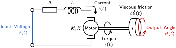
The input is the voltage $v(t)$, the output is the motor rotation angle $\theta (t)$, $i(t)$ is the current, $R$ is the resistance, $L$ is the inductance, $\tau(t)$ is the torque produced by the motor, $K$ is the back electromotive force constant, $M$ is the motor torque coefficient, $J$ is the body inertia moment, and $c$ is the viscous friction coefficient.
First, we derive the equations for the electrical system. The voltage applied to each component can be calculated as follows.
$$\begin{align} \text{Voltage across the resistor}&:Ri \\[3pt] \text{Voltage across the inductor}&:L\dot{i} \\[3pt] \text{Voltage across the motor}&:K \dot{\theta} \end{align}$$
The voltage across the motor represents the back electromotive force produced by the motor rotation. From Kirchhoff’s law, the relation between each voltage is expressed as follows.
$$\text{Equation of Electrical System :} \quad v = Ri + L\dot{i} + K \dot{\theta}$$
Next, we consider the equation of the mechanical system. The equation of motion of the rotating body is expressed as follows.
$$ J \ddot{\theta} = -c \dot{\theta} + \tau$$
The torque generated by the motor is proportional to the current, i.e. $\tau = M i$. Therefore, the equation of motion can be rewritten as follows.
$$\text{Equation of Mechanical System :} \quad J \ddot{\theta} = -c \dot{\theta} + M i$$
In summary, we have
$$ \left\{ \begin{array}{ll}v = Ri + L\dot{i} + K \dot{\theta}& :\ \text{Equation of Electrical System} \\[3pt] J \ddot{\theta} = -c \dot{\theta} + M i& : \ \text{Equation of Mechanical System.}\end{array} \right. $$
Let $V(s)$, $I(s)$, and $\Theta(s)$ be the Laplace transforms of $v(t)$, $i(t)$, and $\theta(t)$, respectively, then the Laplace transform of the above equation becomes
$$ \left\{ \begin{array}{l}V = RI + LsI + K s \Theta\\[3pt] J s^2 \Theta = -c s\Theta + M I.\end{array} \right. $$
From these equations, we can derive the transfer function for the entire system. First, we organize the second equation for $I(s)$.
$$ I = \frac{1}{M} ( Js^2\Theta + cs\Theta )$$
Substitute this into the first equation.
$$\begin{align} V &=\frac{R}{M} ( J s^2\Theta + c s \Theta ) + \frac{L}{M} ( J s^3\Theta + c s^2\Theta ) + K s \Theta \\\\ &= \frac{1}{M} \Bigl\{ LJs^3 + (RJ+Lc)s^2 + (Rc + MK) s \Bigr\}\Theta \end{align}$$
Now we can organize this for the output and get the transfer function.
$$ \Theta = \ubg{ \frac{M}{ LJ s^3 + (RJ+Lc) s^2 + (Rc + MK) s}}{\large \text{Transfer Function}} V$$
Since the degree of $s$ is 3, you can see that the combination of the electrical and mechanical systems makes the overall system third-order. Also, since the denominator of the transfer function can be factored by $s$, we know that one of the poles is zero.
2-DOF Spring-Mass-Damper System
Finally, as an example of combining two mechanical systems, consider the following spring-mass-damper system.

The input is the force $f(t)$ applied to the front cart, the output is the position $x_1(t)$ of the middle cart, $m_1$ and $m_2$ are the masses of the carts, $k_1$ and $k_2$ are the spring constants, and $c_1$ and $c_2$ are the viscosity coefficients. The equations of motion for each cart are expressed as follows.
$$ \left\{ \begin{array}{ll} m_1 \ddot{x}_1 = – k_1 x_1 – c_1 \dot{x}_1 – k_2 (x_1 – x_2) – c_2 (\dot{x}_1 – \dot{x}_2)& :\ \text{Middle Cart} \\[5pt] m_2 \ddot{x}_2 = k_2 (x_1 – x_2) + c_2 (\dot{x}_1 – \dot{x}_2) + f & :\ \text{Front Cart}\end{array} \right. $$
Let $X_1(s)$, $X_2(s)$, and $F(s)$ be the Laplace transforms of $x_1(t)$, $x_2(t)$, and $f(t)$, respectively. Then the Laplace transform of the equation of motion becomes
$$ \left\{ \begin{array}{l} m_1 s^2 X_1 = – k_1 X_1 – c_1 s X_1 – k_2 (X_1 – X_2) – c_2 s(X_1 – X_2) \\[5pt] m_2 s^2 X_2 = k_2 (X_1 – X_2) + c_2 s (X_1 – X_2) + F.\end{array} \right. $$
From these equations, we derive the transfer function for the entire system. By organizing the second equation, we obtain the following:
$$ X_2 = \frac{1}{m_2 s^2 + c_2 s + k_2} \Bigl\{ ( c_2 s + k_2) X_1 + F\Bigr\}$$
Substituting this into the first equation yields the transfer function.
$$ X_1 = \ubg{ \frac{c_2 s + k_2}{\Bigl\{ m_1 s^2 + (c_1 + c_2)s + (k_1 + k_2)\Bigr\} (m_2 s^2 + c_2 s + k_2) – (k_2 + c_2 s)^2} }{\large \text{Transfer Function}} F$$
By organizing the denominator for $s$, we obtain
$$ {\small X_1 = \frac{c_2 s + k_2}{ m_1 m_2 s^4 + \bigl\{m_2 c_1 + (m_1+m_2) c_2\bigr\} s^3 + \bigl\{ m_2 k_1 + (m_1+m_2) k_2 + c_1 c_2 \bigr\}s^2 + (c_1 k_2 + c_2 k_1)s + k_1 k_2} F.}$$
Since the degree of $s$ is 4, we can see that it is a fourth-order system. If there is no spring or damper, we can just set $k$ and $c$ to 0.
Comments